Excel is a powerful tool that helps you manage data efficiently. Applying formatting to cells is one of the essential tasks in Excel. Excel offers many formatting options, including currency, percentage, and date formats. Applying the currency format to cells can be a tedious task, especially when you have to format a large number of cells. Luckily, Excel keyboard shortcuts can make your life easier. In this blog post, we will discuss the Keyboard Shortcut to Apply Currency Format In Excel.
Keyboard Shortcut to Apply Currency Format In Excel
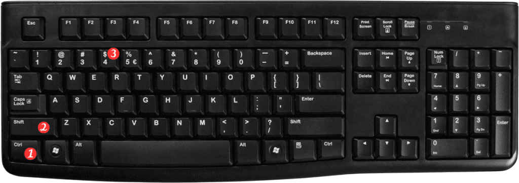
The keyboard shortcut to apply currency format is Ctrl + Shift + $ for Windows and ⌃ + ⇧ + $ for Mac.

Follow the steps below to apply the currency format to cells in Excel:
- Select the cells you want to format.
- Press Ctrl + Shift + $ for Windows or ⌃ + ⇧ + $ for Mac.
That’s it! You have successfully applied the currency format to the selected cells.
Here are a few points to remember about the keyboard shortcut for applying currency format in Excel:
- The keyboard shortcut can be used for both Windows and Mac versions of Excel.
- The currency symbol used in the format will depend on the currency settings of your computer.
- You can also use the Format Cells dialog box to apply currency formatting to cells. The keyboard shortcut to open the Format Cells dialog box is Ctrl+1 for Windows or ⌘+1 for Mac.
- You can customize the keyboard shortcuts in Excel to suit your needs. To do this, go to File > Options > Customize Ribbon > Keyboard Shortcuts and customize the shortcuts as needed.
In conclusion, keyboard shortcuts can save you a lot of time and effort when working with Excel. The keyboard shortcut to apply currency format to cells is Ctrl + Shift + $ for Windows and ⌃ + ⇧ + $ for Mac. So the next time you need to format cells in Excel, try using this keyboard shortcut and see how much time you can save!
