Excel FILTER function is a powerful tool that helps to extract a subset of data from a given range based on specified criteria. This function is particularly useful when working with large data sets and you need to quickly filter out specific information. It can help you to easily analyze, sort and manipulate data by providing a quick and efficient way to filter out irrelevant data.
Excel FILTER Function Summary
Excel’s FILTER function is a powerful tool in the Dynamic Arrays function category that lets you quickly and easily extract data from large datasets based on specified criteria. Simply provide the search criteria as an argument, and the function returns a spill range of matching values. You can even nest it within other functions to perform complex filtering operations.
FILTER Function Purpose
The purpose of the Excel FILTER function is to extract a subset of data from a larger range based on specified criteria. It returns an array of values that meet the specified condition.
FILTER Function Arguments
- array: the range of cells to filter
- include: an array of boolean values or an expression that evaluates to a boolean array, which determines which rows or columns to include in the result
- [if_empty]: optional argument to specify the value returned if no cells meet the specified condition
FILTER Function Return value
The Excel FILTER function returns an array of values that meet the specified condition.
FILTER Function Syntax
=FILTER(array, include, [if_empty])Excel FILTER Function Examples
The Excel FILTER function is a powerful tool for data analysis that allows users to quickly filter a range of data based on specific criteria. With its dynamic array capabilities, FILTER can easily return a range of filtered data that automatically updates as the source data changes. In this section, we will explore some useful examples of how the FILTER function can be used to manipulate and analyze data in Excel.
Basic Excel FILTER Function
In this example, we will use the FILTER function to extract all values in a range that are greater than 5.
You will need the following function:
=FILTER(A2:A11, A2:A11>5)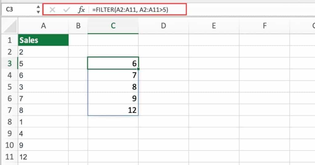
In this example, the FILTER function takes two arguments: the range of data we want to filter (A1:A11), and the criteria we want to filter by (A1:A11>5). This means we want to filter the range A1:A11 to only include values that are greater than 5.
When we enter the formula in cell C3, Excel will automatically spill the results into the cells below. The FILTER function returns only the values that meet the specified criteria, in this case, 6, 7, 8, 9, and 12.
Filtering Data with Multiple Criteria
In this example, we will use the FILTER function to extract all rows that match the criteria “John” in column B of the data set.
=FILTER(B2:E10, B2:B10="John", "Not Found")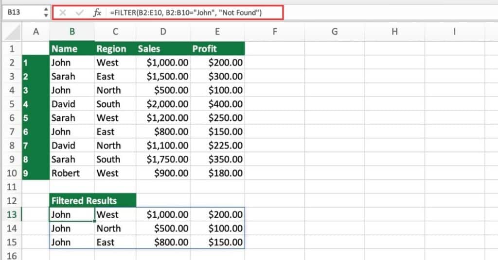
In the FILTER function, we select the entire range B2:E10 as the data range. The second argument is the criteria range, where we specify that we want to filter all rows that have “John” in column B. The third argument is the “Not Found” value, which is displayed in the filtered results when there is no match.
The resulting filtered array is spilled into the range B13:B23, but since we only want to display the filtered results, we use the TRANSPOSE function to display them vertically. The final results are displayed in the range B13:E15 under the heading “Filtered Results”.
Dealing with No Matching Data in Excel FILTER Function
Suppose we want to filter the table to only show the rows where the Gender is “Non-binary”. We can use the FILTER function as follows:
=FILTER(A2:C6, C2:C6="Non-binary", "No matching data")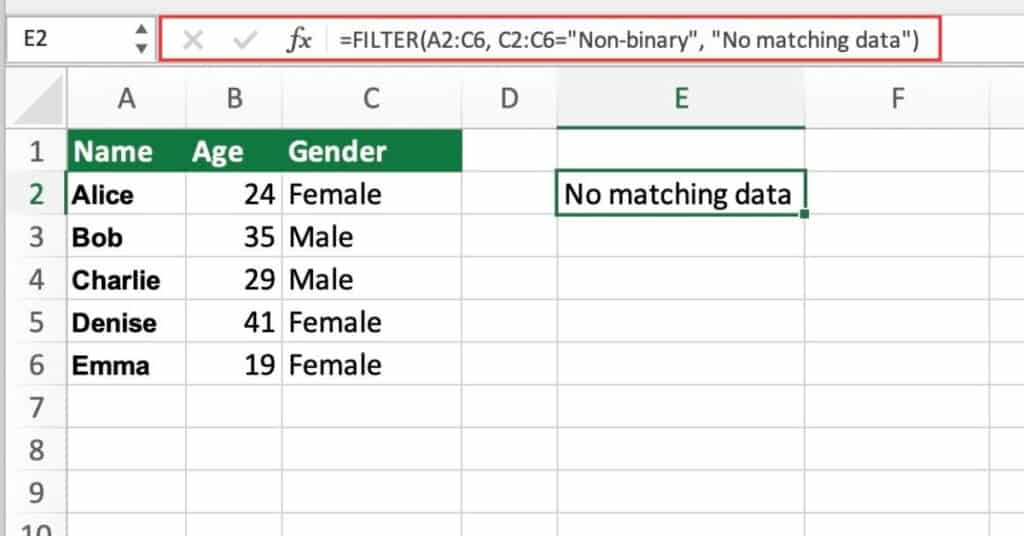
In this case, since there is no row with the Gender “Non-binary”, the function will return the error message “No matching data”.
Note that we specified “No matching data” as the third argument of the function. This is the message that will be displayed when there is no data that matches the criteria.
Filtering Values That Contain Text with Excel’s FILTER Function
I’ll walk through an example of how to use the FILTER function to filter data by text.
In our example, we have a list of products and their corresponding prices in columns A and B. We want to filter the list to only show products that contain the text “ap” in their name.
Here’s the formula we can use:
=FILTER(A2:B11,ISNUMBER(SEARCH("ap",A2:A11)))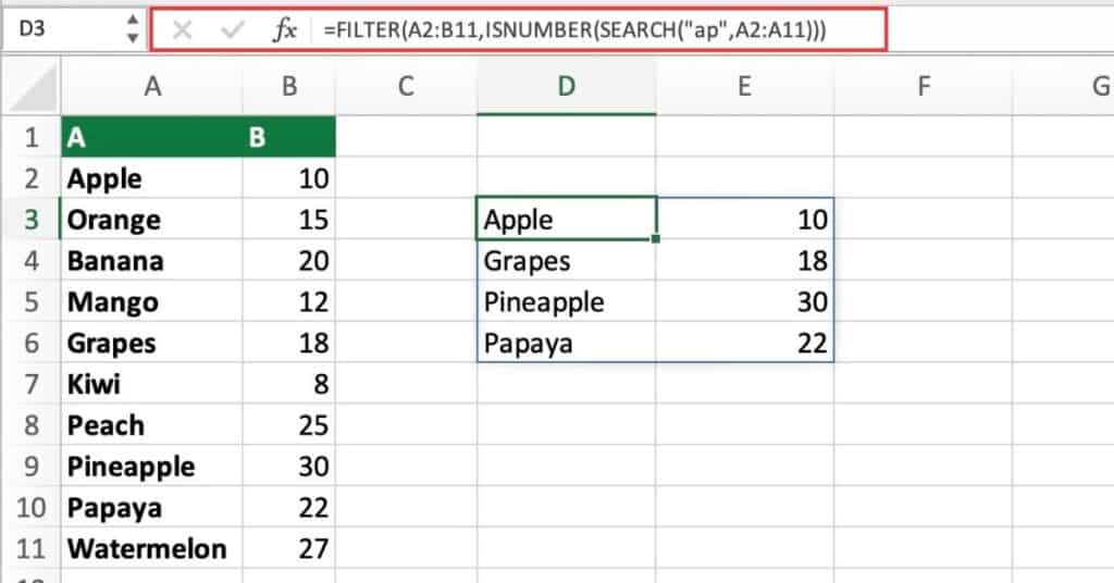
Let’s break down the formula:
- A2:B11 is the range of cells we want to filter.
- ISNUMBER(SEARCH(“ap”,A2:A11)) is the criteria we want to use to filter the data. The SEARCH function searches for the text “ap” within each cell in the range A2:A11. Returning a number if the text is found (and an error if it’s not). The ISNUMBER function then checks if the result of the SEARCH function is a number, which indicates that the text “ap” was found in that cell.
When we enter the formula, it returns a new table with only the rows that meet the filter criteria. In this case, the new table shows only the products that contain the text “ap” in their name, along with their corresponding prices.
Filtering Data by Date with Excel FILTER Function
Suppose you have a table of sales data with three columns: Date, Product, and Sales.
Suppose we want to filter this data to show only the sales that occurred between January 1, 2022, and March 31, 2022.
We can use the FILTER function with the following formula:
=FILTER(A2:C11, A2:A11>=DATE(2022,1,1), A2:A11<=DATE(2022,3,31))This formula uses the FILTER function to filter the table based on the dates in column A.
- The first argument, A2:C11, specifies the range of the table that we want to filter.
- The second argument, A2:A11>=DATE(2022,1,1), specifies the condition that the date must be greater than or equal to January 1, 2022.
- The third argument, A2:A11<=DATE(2022,3,31), specifies the condition that the date must be less than or equal to March 31, 2022.
The resulting filtered table will show only the rows that meet both conditions.
Excel FILTER Function with Multiple Criteria Example
Let’s explore how to use the FILTER function with multiple criteria to filter data from a table based on two or more conditions.
Suppose we want to extract all sales data for Product A that occurred after January 2nd, 2022. We can use the FILTER function with multiple criteria to accomplish this task.
The formula for this would be:
=FILTER(A2:C11, (B2:B11="A")*(A2:A11>DATE(2022,1,2)))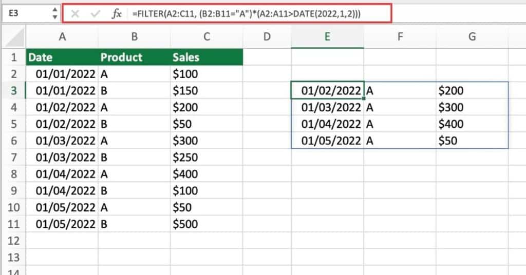
Explanation:
The FILTER function extracts data from the range A2:C11 based on the criteria provided in the second argument of the function.
The first criterion is (B2:B11=”A”), which checks if the product column contains “A”. This will return TRUE for rows where the product is A, and FALSE for rows where the product is B.
The second criterion is (A2:A11>DATE(2022,1,2)), which checks if the date column contains a date that is greater than January 2nd, 2022. This will return TRUE for rows where the date is after January 2nd, and FALSE for rows where the date is on or before January 2nd.
The two criteria are combined using the * (multiplication) operator, which returns TRUE only if both criteria are met.
Filtering Out Blanks with Excel’s FILTER Function
Filtering out blank cells from a large dataset can be a time-consuming task. However, with the FILTER function, you can easily filter out blank cells and display only the relevant data that you need. In this example, we will demonstrate how to use the FILTER function to filter out blank cells in Excel.
To filter out the blank cells in the Age column, you can use the FILTER function with the ISBLANK function. The formula would be:
=FILTER(A2:C10, NOT(ISBLANK(B2:B10)))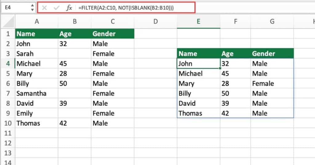
This formula filters the data in columns A to C. Returning only those rows where the Age column is not blank.
As you can see, the blank cells have been filtered out, and only the relevant data remains.
Excel FILTER Function Notes
- The FILTER function is only available in Excel 365 and Excel for the web.
- If the range is not contiguous, the function returns a #SPILL! error.
- The FILTER function may slow down the performance of large data sets.
