In Excel, numbers can be displayed as positive or negative based on their value. Sometimes, you may need to convert negative numbers to positive numbers to simplify your data analysis. This is a common task in financial and accounting applications where you need to calculate absolute values of numbers.
In this blog post, we will learn how to change negative numbers to positive in Excel. This is a simple process that can be accomplished using a formula or formatting options.
How to Change Negative Numbers to Positive in Excel Video
Here’s how to change negative numbers to positive in Excel
Method 1: Paste Special -1
This method is ideal if you want to convert negative values in the same column.
Here’s how you can do it:
Step 1. Select an empty cell and enter -1.
Step 2. Copy the cell with the value -1.
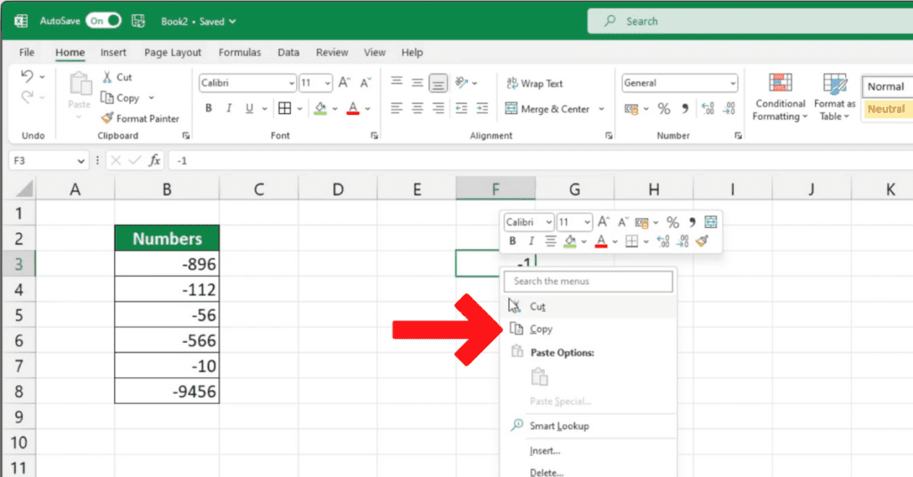
Step 3. Select the column with negative numbers.
Step 4. Right-click and choose ‘Paste Special’
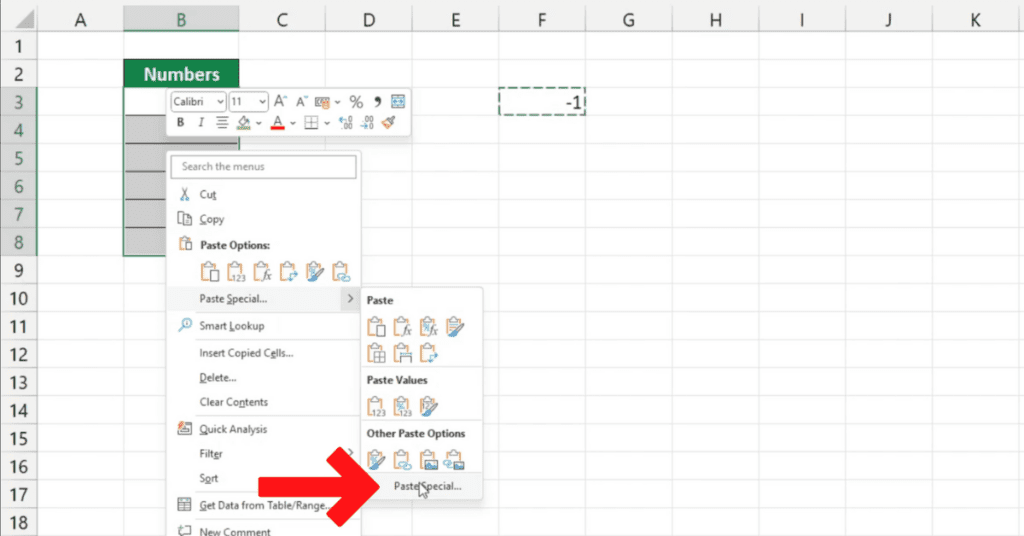
Step 5. In the ‘Paste Special’ window, select ‘Multiply’ and ‘All except borders.’
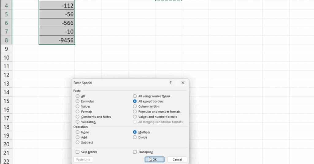
Step 6. Click ‘OK,’ and you’re done.
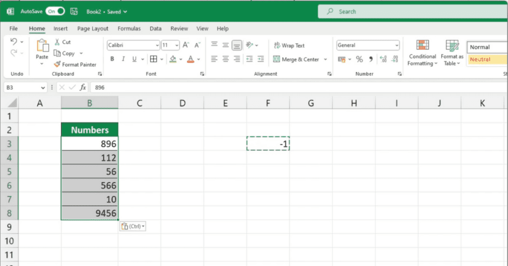
Method 2
The second method is great for creating a new column of positive numbers while keeping the original column intact.
Step 1. To get started, first, select the cell where you want to enter the formula.
Step 2. This cell should be in the column where you want to display the positive numbers.
Step 3. Next, type the equal sign (=) to begin the formula, then select the cell containing the negative value that you want to turn into a positive.
Step 4. Finally, multiply the value by -1.
Here’s an example formula:
=A2*(-1)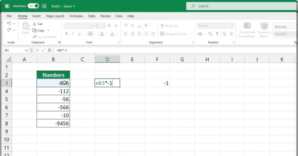
In this example, the negative number is in cell A2.
The formula will multiply the value by -1, which will turn the negative value into a positive one.
Step 5: Once you’ve entered the formula, hit enter, and the positive number will appear in the selected cell.
If you need to change all the values in the column, simply copy the formula by selecting the cell, and then dragging the formula down to all the rows that contain negative numbers.
And that’s it! You’ve successfully converted negative numbers to positive ones using a formula in Excel.
Method 3
Step 1. Select the cell or range of cells that contains the negative numbers you want to convert.
Step 2. Press “Ctrl + 1” to open the Format Cells dialog box.
Step 3. In the Format Cells dialog box, go to the Number tab and select “Custom” from the Category list.
Step 4. In the Type field, enter the following formula: 0;-0
Step 5. Click OK to close the dialog box.
Excel will now display all negative numbers as positive numbers in the selected cell or range of cells. If you want to apply this formatting to other cells, you can use the Format Painter tool to copy the formatting to other cells.
Congratulations! You’ve just learned three effective ways to turn negative numbers into positive ones in Excel.
Here are some bullet points to keep in mind:
- Before you convert negative numbers to positive ones, make sure you understand the impact of the change on your data.
- If you want to convert negative numbers in the same column, Method 1 (Paste Special -1) is the best option. If you want to create a new column of positive numbers, Method 2 (Formula) is the way to go.
- If you want to change the way negative numbers are displayed without actually changing the values, Method 3 (Formatting) is a good choice.
- Always make sure to double-check your work after converting negative numbers to positive ones.
- If you’re working with large data sets, consider using Excel’s built-in filters or sorting tools to help you locate negative numbers quickly.
Finally, remember that Excel is a powerful tool that offers many different ways to manipulate data. Don’t be afraid to experiment and try new things when learning Excel!
