Counting the number of items that fall within a certain range is a common task in data analysis. In Excel, you can easily count the number of items between two numbers using the COUNTIFS function. In this post, we’ll go over the steps to use the COUNTIFS function to count between two numbers in Excel.
Guide to Counting Between Two Numbers in Excel
Open your Excel worksheet and select the cell where you want the count to appear.
Enter the following formula into the cell.
=COUNTIFS(range1,">"&number1,range2,"<"&number2)Replace “range1” and “range2” with the ranges of cells you want to count between.
Replace “number1” and “number2” with the numbers that define your range.
Press Enter to calculate the result.
What’s Happening with the Function?
The COUNTIFS function counts the number of items in one or more ranges that meet multiple criteria.
In this case, we’re using two criteria. The numbers in the range must be greater than “number1” and less than “number2.”
The “&” symbol concatenates the “>” or “<” symbol with the number, so we’re comparing the values in the range to those two criteria.
The result is the number of items that fall within the specified range. Things to Keep in Mind Make sure that the ranges you specify in the formula are valid and include only the cells you want to count between.
Double-check that you’re using the correct comparison operators (“>” and “<“) and that they’re in the correct order.
You can use the COUNTIF function to count items that meet only one criterion.
Count Between Two Numbers in Excel Example
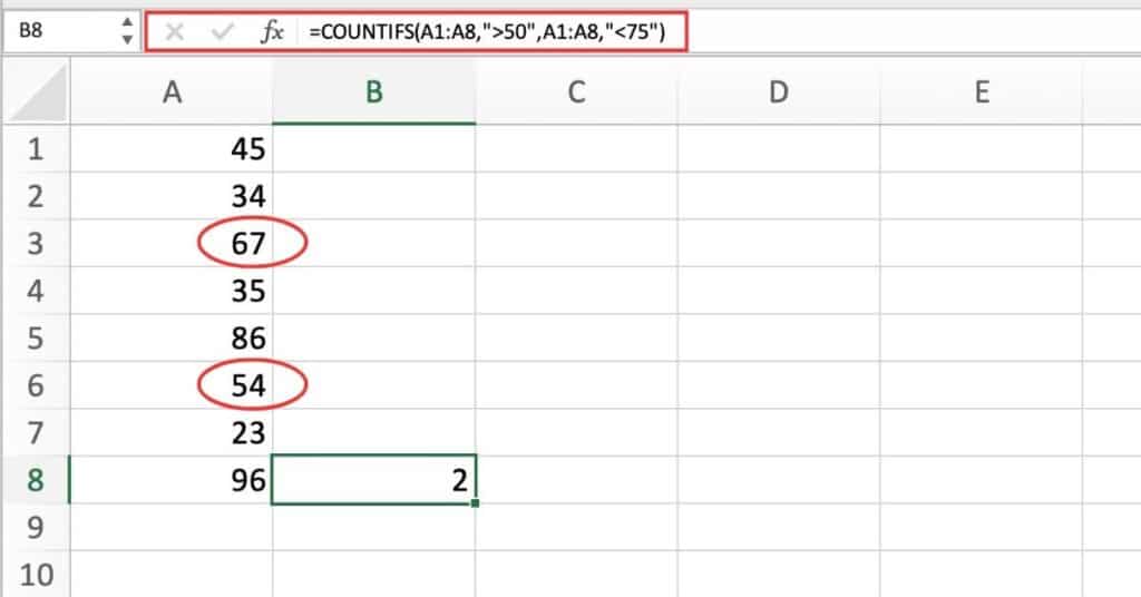
Suppose you have a range of numbers in column A, and you want to count how many numbers fall between 50 and 75.
You can use the following formula:
=COUNTIFS(A1:A8,">50",A1:A8,"<75")This formula counts the number of cells in column A that meet two criteria. The value in the cells must be greater than 50, and the value in the cells must be less than 75.
Here’s a breakdown of the formula:
- “COUNTIFS” is the function we’re using to count the number of cells that meet multiple criteria.
- “A:A” refers to the range of cells we want to count. In this case, we want to count all the cells in column A.
- “>50” is the first criteria we’re using. We’re asking Excel to count all cells that are greater than 50.
- “<75” is the second criteria we’re using. We’re asking Excel to count all cells that are less than 75.
You can modify this formula to count values between any two numbers by changing the criteria in the formula.