Excel Ribbon | Complete Guide

Microsoft Excel is a powerful spreadsheet program that allows users to organize, analyze, and present data in a variety of ways. The Excel Ribbon is the primary interface for accessing the program’s features and functions. 

The Ribbon consists of a series of tabs that group related commands and features. 

In this blog post, we’ll explore the Excel Ribbon Tabs and Groups to help you better understand how to navigate and use Excel.

Excel Ribbon

Microsoft Excel ribbon is the row of tabs and icons at the top of the Excel window that allows you to quickly find, understand and use commands for completing a certain task. It looks like a kind of complex toolbar, which it is. 

The ribbon first appeared in Excel 2007 replacing the traditional toolbars and pull-down menus found in previous versions.

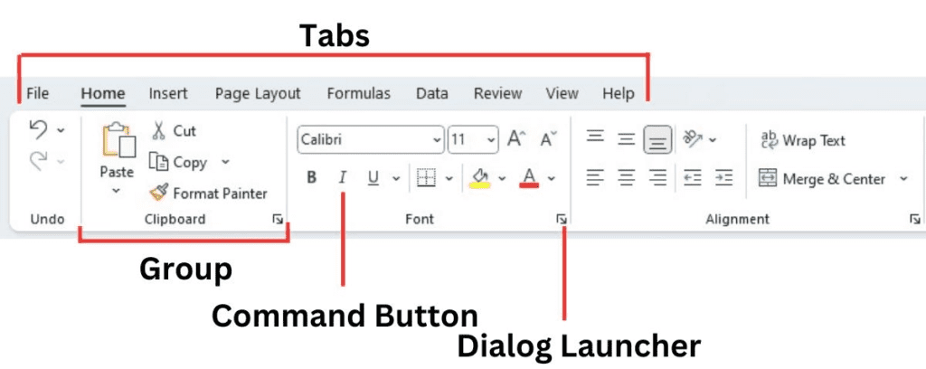
In Excel 2010, Microsoft added the ability to personalize the ribbon. The ribbon in Excel is made up of four basic components: tabs, groups, dialog launchers, and command buttons.

Excel Ribbon: A UI element with tabs containing groups of related commands.

Ribbon tab: A category of related commands on the Ribbon.

Ribbon group: A subset of commands within a Ribbon tab for a specific task.

Dialog launcher: A small arrow icon in a Ribbon group that opens a dialog box with more options.

Command button: An icon or label on the Ribbon that executes a specific command.

The Ribbon Tabs

The Excel Ribbon is divided into several tabs that are displayed at the top of the program window. 

Each tab is labeled with a name that corresponds to a particular set of commands and features. 

The default tabs in Excel are:

• Home: This tab contains the most frequently used commands such as formatting, editing, and viewing options. It is also where you can access the Clipboard, Font, Alignment, and Number groups.
• Insert: This tab allows you to add various objects such as charts, tables, pictures, and more. You can also use this tab to insert different types of text, symbols, and equations.
• Page Layout: This tab contains options for page setup, including orientation, margins, and page background. You can also access themes, page borders, and other formatting options in this tab.
• Formulas: This tab provides access to different types of formulas, functions, and equation builders.
• Data: This tab allows you to import, sort, filter, and analyze data. You can also use this tab to group, subtotal, and create PivotTables.
• Review: This tab contains options for proofreading, comments, protection, and changes tracking.
• View: This tab contains different options for viewing the worksheet, such as zoom, gridlines, and window arrangement. You can also access the Macros and Workbook Views groups in this tab.

The Ribbon Groups

Each tab on the Excel Ribbon is further divided into groups that contain related commands and features. 

The groups are arranged from left to right and are labeled with a name that indicates their purpose. 

Some of the common groups you’ll find in Excel include:

• Clipboard: This group contains commands for copying, pasting, and cutting data.
• Font: This group contains options for changing the font, font size, and font style.
• Alignment: This group contains options for aligning text and objects within cells.
• Number: This group contains options for formatting numbers, including currency, percentage, and decimal places.
• Charts: This group contains options for creating different types of charts such as bar, line, and pie charts.
• Tables: This group contains options for creating and formatting tables.
• Symbols: This group contains options for inserting different types of symbols, including special characters, mathematical symbols, and emojis.
• Formulas: This group contains options for creating and editing formulas and functions.
• Sort & Filter: This group contains options for sorting and filtering data.
• PivotTable: This group contains options for creating and managing PivotTables.
• Comments: This group contains options for adding, viewing, and editing comments.

How to Hide the Ribbon in Excel

The Excel Ribbon is a powerful tool that provides quick access to a wide range of features and commands. 

However, there may be times when you want to hide the Ribbon to free up more screen space or to minimize distractions while working on a project. Here’s how to hide the Ribbon in Excel:

• Double-Click on Any of the Ribbon Tabs

One way to hide the Ribbon is to double-click on any of the tabs located at the top of the Excel window. Doing so will minimize the Ribbon, showing only the tab names. To restore the Ribbon, simply double-click on any of the tabs again.

• Click on the Upward-Facing Arrow Icon

Another way to hide the Ribbon is to click on the upward-facing arrow icon located on the right-hand side of the Ribbon. This will hide the Ribbon, showing only the tab names. To restore the Ribbon, simply click on the same arrow icon again.

• Hide Ribbon in Excel With Keyboard Shortcut

You can also hide the Ribbon by pressing the Ctrl + F1 keys on your keyboard. This will hide the Ribbon and show only the tab names. To restore the Ribbon, simply press the same key combination again.

Note that when the Ribbon is hidden, you can still access all the commands and features by clicking on the tab names or by using keyboard shortcuts.

Hiding the Ribbon is a useful way to free up more screen space and to focus on the task at hand. So, the next time you want to work on an Excel project without any distractions, try hiding the Ribbon using one of these methods.

How to Unhide Ribbon in Excel

If you’ve previously hidden the Ribbon in Excel, it’s easy to bring it back whenever you need it. Here’s how to unhide the Ribbon in Excel:

• Double-Click on Any of the Tab Names

If you’ve hidden the Ribbon by double-clicking on any of the tab names, simply double-click on any of the tabs again to bring the Ribbon back.

• Click on the Downward-Facing Arrow Icon

If you’ve hidden the Ribbon by clicking on the upward-facing arrow icon located on the right-hand side of the Ribbon, simply click on the same arrow icon again. This will bring the Ribbon back.

• Unhide Ribbon in Excel With Keyboard Shortcut

If you’ve hidden the Ribbon by pressing the Ctrl + F1 keys on your keyboard, simply press the same key combination again to bring the Ribbon back.

Once you’ve unhidden the Ribbon, it will remain visible until you decide to hide it again. If you want to free up more screen space, you can always hide the Ribbon again using one of the methods described in the previous section.

How to Customize Excel Ribbon

The Excel Ribbon is a powerful tool that provides quick access to a wide range of features and commands. 

However, you may find that certain commands that you use frequently are buried within tabs or groups that you don’t use as often. 

Fortunately, Excel allows you to customize the Ribbon to make it work better for you. 

Here’s how to customize the Excel Ribbon:

Customize Excel Ribbon

To get started, right-click on the Ribbon and select “Customize the Ribbon” from the context menu. This will bring up the Excel Options dialog box, with the Customize Ribbon tab selected.

Add or Remove Tabs

On the Customize Ribbon tab, you’ll see two lists of tabs: the Main Tabs list and the Customize the Ribbon list.

The Main Tabs list contains the default tabs that are always visible, while the Customize the Ribbon list contains all the available tabs that you can add or remove from the Ribbon.

To add a tab to the Ribbon, select it in the Customize the Ribbon list and click on the “Add” button.

To remove a tab from the Ribbon, select it in the Main Tabs list and click on the “Remove” button.

Add or Remove Groups

Within each tab, you’ll see several groups of commands. You can also customize these groups by adding or removing commands.

To add a command to a group, select the group in the Main Tabs list and click on the “New Group” button.

This will create a new group within the tab, which you can then customize by adding commands from the list on the right-hand side of the dialog box.

To remove a command from a group, select the group in the Main Tabs list, select the command in the list below, and click on the “Remove” button.

Rename or Reorder Tabs and Groups

You can also rename or reorder tabs and groups to make them easier to find and use. To rename a tab or group, select it in the Main Tabs list, click on the “Rename” button, and enter a new name.

To reorder tabs and groups, select the tab or group in the Main Tabs list and click on the “Up” or “Down” button to move it up or down the list.

Once you’ve customized the Ribbon to your liking, click on the “OK” button to save your changes.

When learning to use Excel the ribbon will be something you use a lot. Getting it customized to best suit your workflow will make tasks easier and quicker. Remember the changes are not permanent and you can keep changing the ribbon to suit what you are working on.