The HLOOKUP function is a lookup and reference function in Excel that allows you to search for a value in the first row of a table or range of cells, and then return a corresponding value in the same column from a specified row. It is commonly used to retrieve data from a table that is organized horizontally. The H in HLOOKUP stands for “horizontal,” indicating that the function performs a horizontal lookup. By using the HLOOKUP function, you can easily find and retrieve data from a large table or range of cells without having to manually search for the value.
Excel HLOOKUP Function Summary
Excel’s HLOOKUP function searches for a value in the first row of a table and retrieves data from a specific row based on a given condition in the same column. Learn how to use this powerful tool for efficient data retrieval.
HLOOKUP Function Purpose
The HLOOKUP function is used to search for a value in the first row of a table or range of cells and then return a corresponding value from a specified row in the same column.
HLOOKUP Function Arguments
The HLOOKUP function takes four arguments:
- lookup_value: This is the value that you want to search for in the first row of the table or range of cells.
- table_array: This is the range of cells or table containing the data that you want to search.
- row_index_number: This is the row number within the table or range from which you want to return a value. The row number is relative to the table or range, not the worksheet.
- [range_lookup]: This is an optional argument that specifies whether you want an exact match or an approximate match to the lookup value. If omitted or set to TRUE, an approximate match is returned. If set to FALSE, an exact match is required.
HLOOKUP Function Return value
The HLOOKUP function returns the value from the specified row and column of the table or range. If an exact match is not found, the function returns the closest match that is less than the lookup value when the range_lookup argument is set to TRUE.
HLOOKUP Function Syntax
The syntax for the HLOOKUP function is as follows:
=HLOOKUP(lookup_value, table_array, row_index_number, [range_lookup])Here’s a brief explanation of each argument:
- lookup_value: The value you want to find.
- table_array: The range of cells that contains the table.
- row_index_number: The row number in the table from which you want to return a value.
- range_lookup (optional): Determines whether the lookup value needs to be an exact match or not. Set to TRUE or omitted for an approximate match, or set to FALSE for an exact match.
HLOOKUP Approximate Match Example
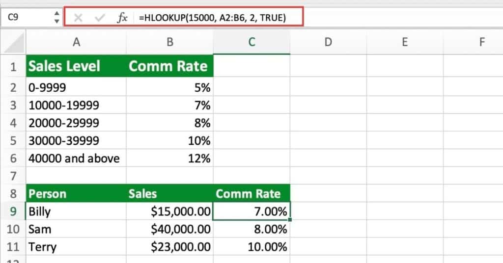
Suppose we have a table that shows the commission rate for different sales levels.
Now, let’s say we want to find the commission rate for a salesperson who made $15,000 in sales. We can use the HLOOKUP function to find the commission rate as follows:
=HLOOKUP(15000, A2:B6, 2, TRUE)
In this formula, 15000 is the lookup value, A1:B6 is the table range, 2 is the row index number (which is where the commission rate is located in the table), and TRUE specifies that we want an approximate match.
The function will return 7%, which is the commission rate for sales between 10000-19999, the closest sales range below 15000.
HLOOKUP Exact Match Example
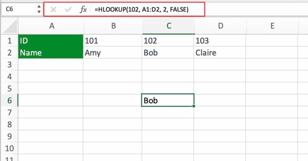
Suppose we have a table of employee information, with employee IDs in the first row and the corresponding employee names in the second row:
If we want to find the name of the employee with ID 102, we can use the HLOOKUP function with an exact match by setting the “range_lookup” argument to FALSE. The formula would be:
=HLOOKUP(102, A1:D2, 2, FALSE)
This formula would search for the value 102 in the first row of the table (range A1:D2) and return the value in the second row of the corresponding column, which is “Bob”. Since we specified an exact match, the function will only return a result if it finds a value that matches exactly with the lookup value.
Using HLOOKUP with Other Excel Functions
HLOOKUP is a useful Excel function that can be combined with other functions to create more powerful formulas. Here are a few examples.
Using HLOOKUP with IF function
You can use the IF function with HLOOKUP to specify different results based on certain conditions. For example, you could use the following formula to check if a certain value is greater than a threshold value and return a corresponding result:
=IF(HLOOKUP("Threshold", A1:F2, 2, FALSE) < 100, "Below Threshold", "Above Threshold")Using HLOOKUP with SUM function
You can use the HLOOKUP function with the SUM function to add up all the values in a row that meet certain criteria. For example, you could use the following formula to sum up all the sales figures for a particular product:
=SUM(HLOOKUP("Product A", A1:F5, {2,3,4}, FALSE))Using HLOOKUP with INDEX and MATCH functions
You can use the INDEX and MATCH functions with HLOOKUP to retrieve a specific value from a table. For example, you could use the following formula to retrieve the value in row 2 and column 3 of a table:
=INDEX(A1:F2, MATCH("Row 2", A1:A2, 0), HLOOKUP("Column 3", A1:F1, 1, FALSE))By combining HLOOKUP with other Excel functions. You can create more complex formulas that can help you analyze and manipulate your data more efficiently.
Tips for using the HLOOKUP function in Excel
- HLOOKUP searches for a value in the first row of a table and retrieves data from a specific row.
- It’s useful for finding data in large tables.
- HLOOKUP can only search from left to right in a table. The search value must be located in the first row of the table.
- If an exact match is not found, HLOOKUP can return an approximate match based on the next closest value.
- It requires four arguments: lookup_value, table_array, row_index_num, and [range_lookup].
