Excel is a powerful tool for organizing and analyzing data. One of the most useful features in Excel is the ability to create filters, which allow you to quickly sort and display data that meets certain criteria. In this tutorial, we will walk you through how to create a filter in Excel.
How to Create Filter in Excel Video
Step-by-Step Guide: How to Create a Filter in Excel
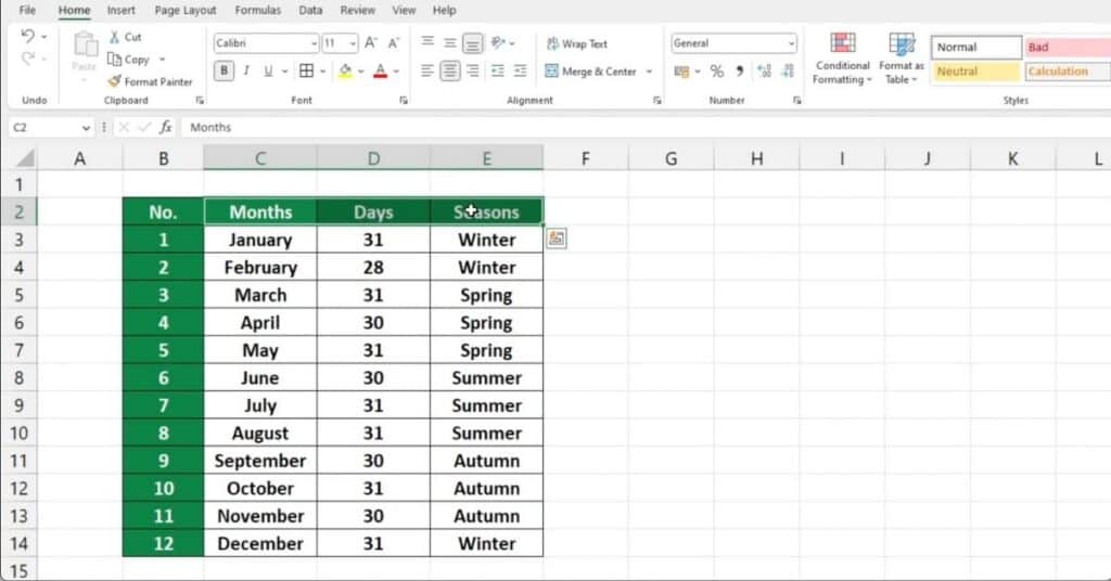
Step 1. Open the Excel spreadsheet that you want to filter.
Step 2. Select the range of cells that you want to filter.
Step 3. This could be a single column or multiple columns.

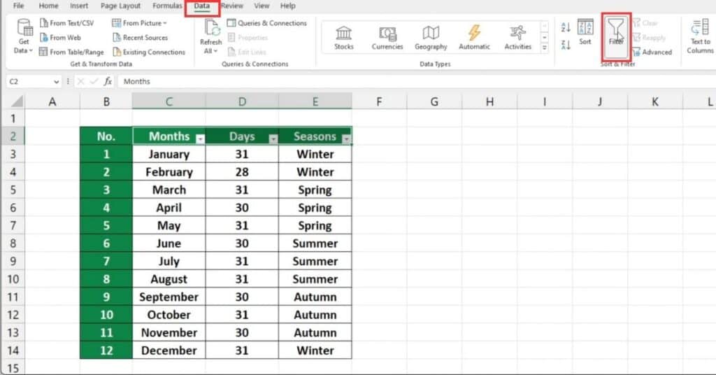
Step 4. Click on the “Filter” button in the “Sort & Filter” group on the “Data” tab.

Step 5. Excel will add a filter drop-down arrow to each column header.
Step 6. Click on the drop-down arrow for the column that you want to filter.
Step 7. In the drop-down menu, select the criteria that you want to filter by.

For example, you can choose to only show values that are greater than or less than a certain number, or you can choose to show values that contain a certain text string.
Excel will filter the data based on your criteria and only show the rows that meet the selected criteria.
Things to Keep in Mind
- Excel allows you to filter multiple columns at once. Simply repeat the process for each column that you want to filter.
- You can also use the “Sort” function in conjunction with filters to sort the filtered data in ascending or descending order.
- Filters are dynamic, which means that if you change the data in the spreadsheet, the filter will automatically update to reflect the changes.
- Be careful when working with filtered data, as it can be easy to accidentally delete or modify data that you didn’t intend to. Always make sure to double-check your work before making any changes.
Finally, remember that Excel is a powerful tool that offers many different ways to manipulate data. Don’t be afraid to experiment and try new things when learning Excel!
