In this short tutorial, I’m here to show you a simple way How to Freeze Rows in Excel.
Freezing rows and columns in Excel can be incredibly helpful, especially when dealing with large tables of data.
How to Freeze Rows in Excel Video
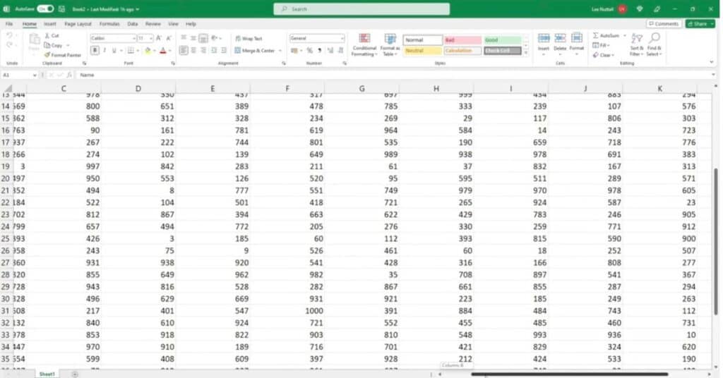
Example of Unfrozen Rows & Columns in Excel
Let’s take a look at an example.
If you scroll down or across the spreadsheet, you might notice that the header (in this case the months) and the column with the employees’ names disappear.

This makes it hard to keep track of the data.
To make it easier to read, we can use the ‘Freeze Panes’ function.
How to Freeze First Row & Column in Excel
First, click on the cell which marks the rows and columns that you want to freeze.
Here, we are freezing the first row and the first column, so we click on cell B2.
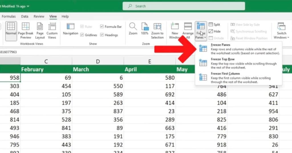
After marking the cell, click on the tab ‘View’, then go to the section ‘Window’ and select ‘Freeze Panes’.

This will lock the header and the column with employees’ names in their position on the screen.
How to Unfreeze Rows & Columns in Excel
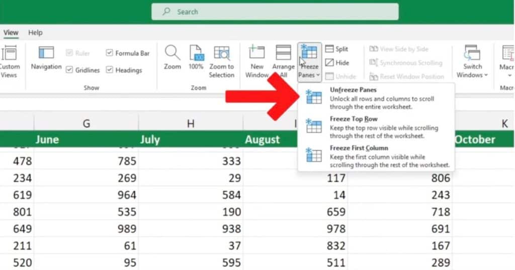
To undo this formatting change, go back to the ‘View’ tab, and in the section ‘Window’ select the option ‘Unfreeze Panes’.
This will remove the formatting change and ‘unlock’ the row and column so that they disappear when you scroll down or across to the right.

If you want to know How to Merge Cells in Excel, read our other tutorial.
If you found this tutorial helpful, and if you want to learn Excel our complete guide section is the place to go that will help you use Excel like a boss!
Want to learn how functions work in excel then check out my excel functions page where you will learn many of the functions. Or looking for formulas? Well, we have you covered there too with our Excel Formulas page.
