In this tutorial I’ll be showing you a simple way How to Multiply Numbers in Excel.
With this table as an example, you’ll learn how to work out anything you need, step by step.
How to Multiply Numbers in Excel Video
How to Multiply Numbers in Excel
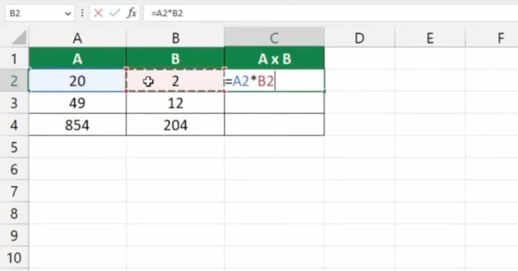
First, click on the cell in which you want to display the result – let’s select cell C2 for our first calculation.
Now, find the ‘equal‘ key and press it.
This tells Excel that you’re about to enter a formula in the cell.
Then, click on the cell that contains the first number to be multiplied – in this case it’s cell A2.
You’ll see another part of the formula will appear after the ‘equal’ sign – it’s the cell reference, A2.
Next, add the symbol for the mathematical operation you want to carry out.
In this case, you’ll use an asterisk, which is used for multiplication in Excel.
Then, click the cell that contains the multiplier – B2.

Now you’ve told Excel to multiply the number in A2 with the number in B2 – hit ‘Enter‘ and you’re done!
The result is available at once.
You can use similar steps to add, subtract or even divide in Excel.
Using the Fill Handle to Copy Multiply Formula
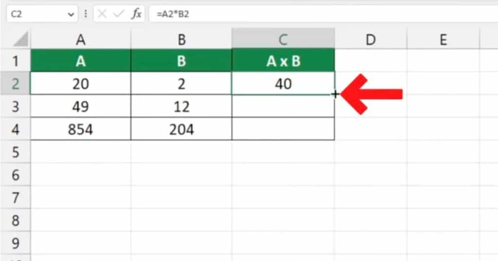
And here comes a handy little ‘trick’ just for you – if you need to multiply the numbers in rows 3 and 4, click on the cell containing the formula we’ve just created – which is cell C2.
Then, hover over the bottom right corner of the cell until you see a cross symbol, and use left-click to drag the formula down through the rest of the rows.

And that’s it – you’ve multiplied the numbers in all three rows!
If you want to know Add, Subtract, or Divide read our other tutorial.
If you found this tutorial helpful, and if you want to learn Excel our complete guide section is the place to go that will help you use Excel like a boss!
Want to learn how functions work in excel then check out my excel functions page where you will learn many of the functions. Or looking for formulas? Well, we have you covered there too with our Excel Formulas page.
