How to Unhide Rows in Excel | Beginner’s Guide

Welcome to Sheet Leveller! In this tutorial, I’ll show you some easy steps on how to unhide rows in Excel, which will show the data in these rows.

So let’s have a look at it!

In the last lesson, we learned how to hide rows in Excel.

Now, let’s turn our attention to how to unhide them.

How to Unhide Rows in Excel

Watch this video on YouTube.

Identifying Hidden Rows In Excel

Usually, it’s not hard to identify rows that have been hidden in a worksheet.

One method for locating them is to search for a double line, similar to this one, among the row headings.

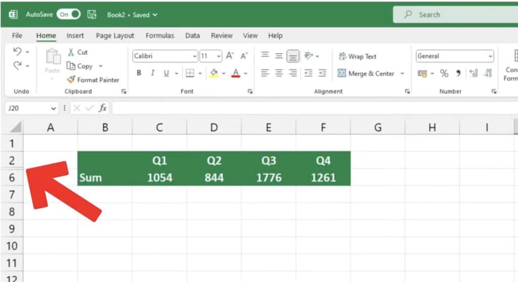
A skipped order of numbers can be indicative of rows being hidden.

Typically, the numbers progress in a sequence of 1,2,3,4, and so on.

In this case, rows 4, 5, and 6 have been hidden, as we see row 7 right below row 3.

It’s time to learn two simple ways to unhide rows.

Unhide Rows in Excel With the Mouse

Here is the first way we will look at it!

First, you must choose the rows you wish to make visible.

To unhide rows in a spreadsheet, select the row immediately above and below the hidden rows that you wish to unhide.

To make hidden rows visible again, right-click and select the Unhide option.

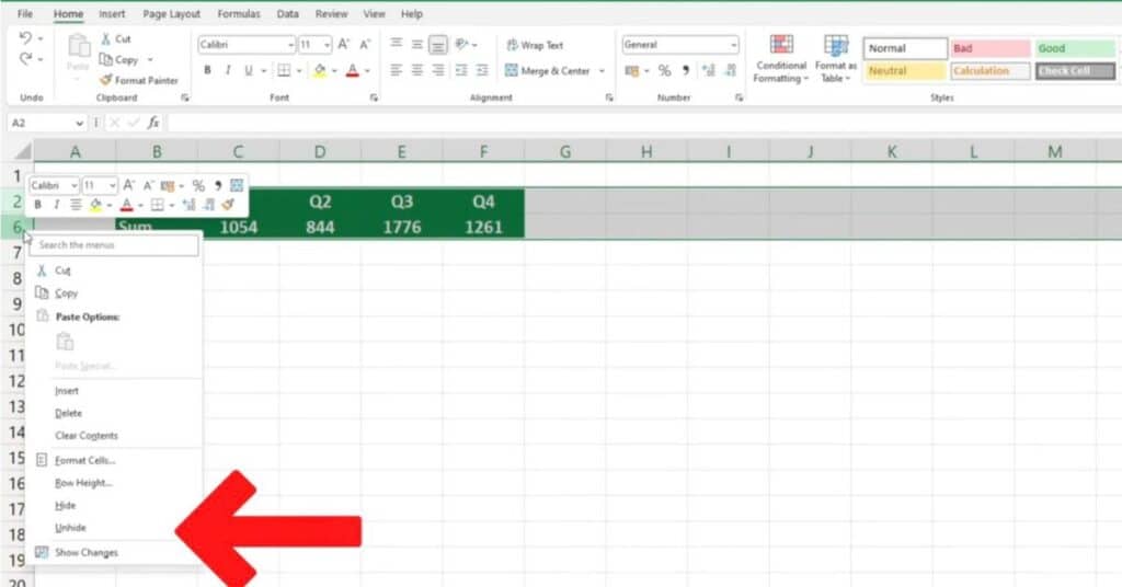
These rows will then be displayed in the table on the screen and will also be included in the printed sheet.

We’ll now undo the changes to take a look at the second method for uncovering rows in Excel.

Unhide Rows in Excel With the Ribbon

Select the row(s) as we did earlier.

Now, to unhide the selected rows, we can go to the Home tab, go to the Cells section, click Format, then select the Hide & Unhide option from the menu, and click Unhide Rows.

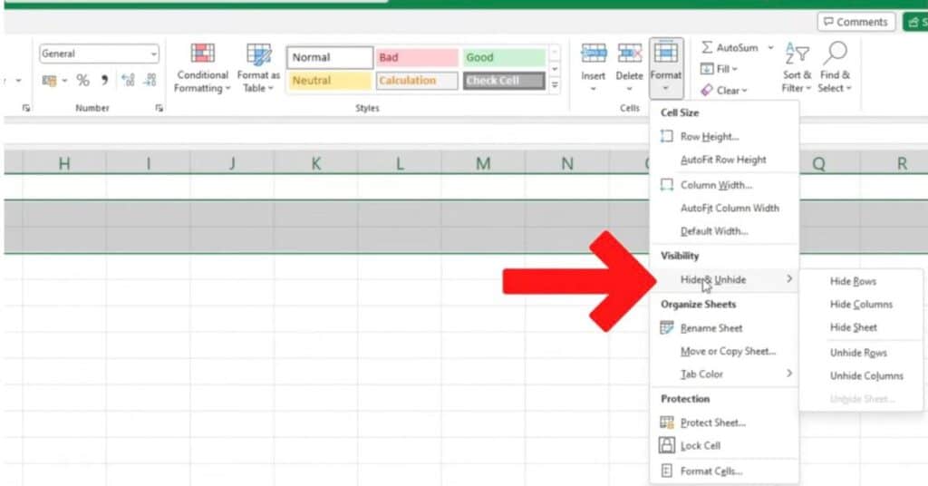
Great, we’re almost done here.

I have two helpful tips to share with you.

How to Unhide the First Row in Excel

First, if the hidden row is the first row of the spreadsheet (row 1), you will need to first select row 2 (the row immediately below it) and then highlight the column headings (containing letters) above.

This will allow you to highlight the hidden row 1 from both sides, and then you can easily unhide it.

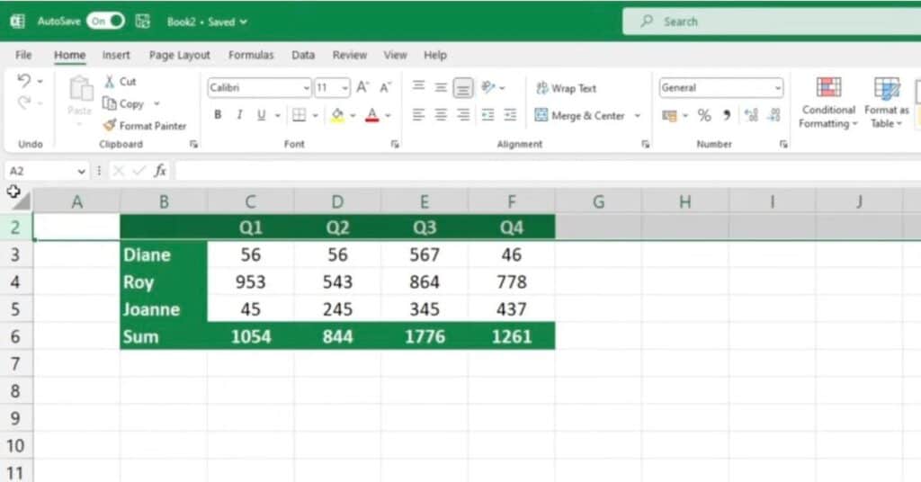
There is one more way how we can achieve this let’s take a look.

Unhide All Rows in Excel

Now, if you want to unhide all rows in the whole spreadsheet, click on the top left-hand corner.

This will highlight the entire sheet.

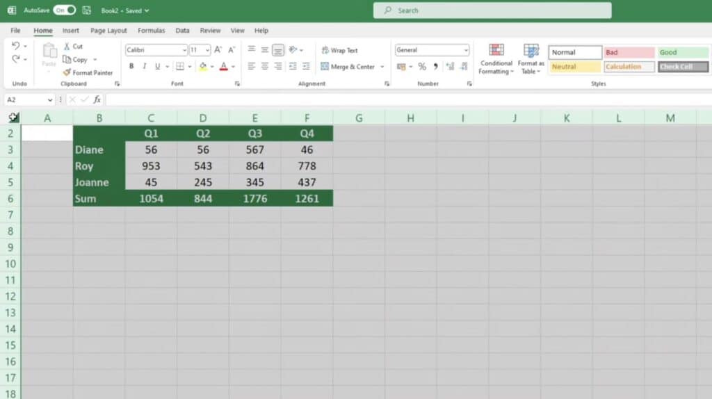
Right-click on the row headings, select the Unhide option, and all rows will become visible.

And there you have it!

You have successfully learned How to Unhide Rows in Excel.

If you found this tutorial helpful, and if you want to learn Excel our complete guide section is the place to go that will help you use Excel like a boss!

You will find many other tutorials including How to Hide Rows in Excel.

You can also read more tutorials that help you use Excel Like A Boss!

If you like YouTube to take in your Excel knowledge then check out my YouTube channel Sheet Leveller.

Thanks for reading. See you in the tutorial!