Excel INDEX function is a powerful tool that helps in finding and returning a specific value from a table or a range of cells. It allows you to extract data from a specified area of your worksheet by referencing its position or location.
Excel INDEX Function Summary
Discover how to extract values or references from a table or range using the versatile INDEX function. Learn how to use the two different forms of the function: the Array form for returning the value of a specific cell or array of cells, and the Reference form for returning a reference to specified cells. Take your Excel skills to the next level with INDEX.
Excel INDEX Purpose
The main purpose of the Excel INDEX function is to retrieve the value of a cell in a specific row and column within a range of cells.
Excel INDEX Arguments
The INDEX function has two main arguments: array and row_num or column_num. The array argument is the range of cells that contains the value you want to retrieve. The row_num and column_num arguments are the row and column coordinates of the cell that contains the value you want to retrieve.
Excel INDEX Return Value
The Excel INDEX function returns the value of a cell based on the row_num and column_num arguments. It can return a single value or an array of values.
Excel INDEX Syntax
The syntax for the INDEX function is as follows:
=INDEX(array, row_num, [column_num])Excel INDEX Function Examples
To help you better understand how to use the INDEX function, let’s take a look at a few examples. In these examples, we will use both the array and reference forms of the INDEX function to retrieve data from a table or range.
Retrieve a single value from a table
Suppose you have a table of data with column headers and row labels, and you want to retrieve the value in cell C4. You can use the INDEX function as follows:
=INDEX(B2:E8,3,2)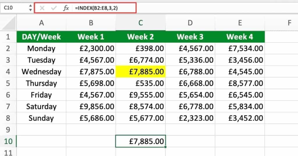
Here’s what’s happening with the formula:
- INDEX: This is the name of the function that we are using.
- C2:F6: This is the range or array from which we want to retrieve the data.
- 3: This is the row number within the range where we want to retrieve the data. In this case, we are selecting the third row.
- 2: This is the column number within the range where we want to retrieve the data.
In this case, we are selecting the second column. So, the formula is essentially telling Excel to retrieve the value that is located in the third row and second column of the range C2:F6. So in our example here the cell will be C4.
Retrieve multiple values from a table
Suppose you want to retrieve all the values in a specific column or row of a table.
You can use the INDEX function with an array formula to retrieve all the values in a column as follows:
=INDEX(B2:F6, , 3) (to retrieve all values in column C)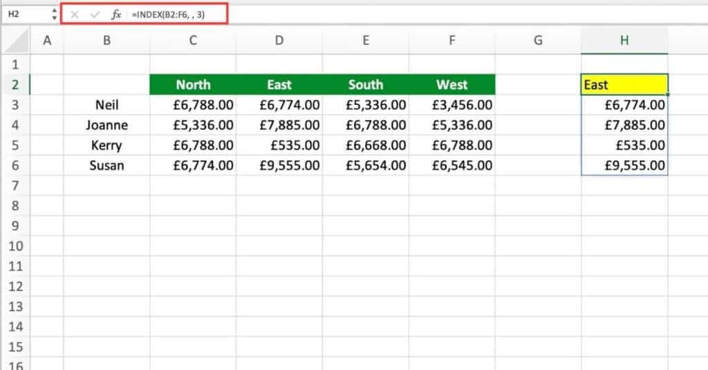
You can use the INDEX function with an array formula to retrieve all the values in a rows as follows:
=INDEX(B2:F6, 3, ) (to retrieve all values in row 3)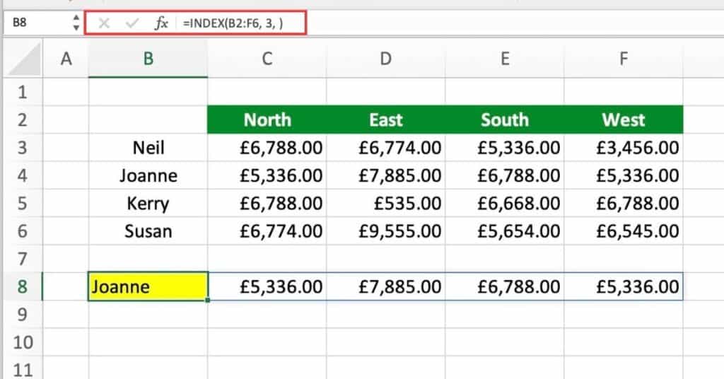
INDEX and MATCH
Suppose you have a table that shows the sales figures for different products in different regions, and you want to find the sales figure for a specific product in a specific region. You can use the INDEX and MATCH functions together to do this.
Here’s the formula you can use:
=INDEX(C2:F6,MATCH(D8,B2:B6,0),MATCH(E8,C2:F2,0))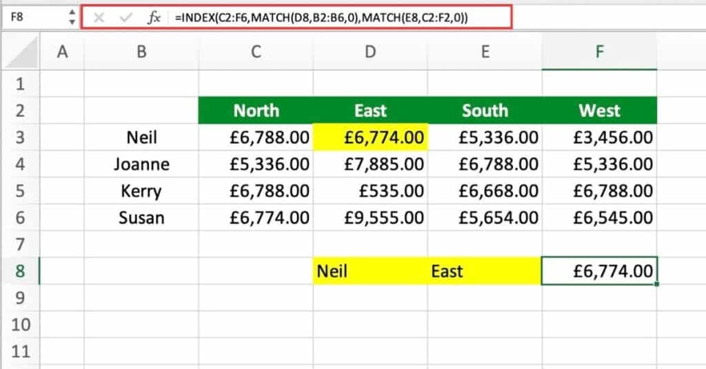
Let’s break down what’s happening in this formula:
- The INDEX function is used to return a value from a specified range. In this case, the range is C2:F6.
- The MATCH function is used to find the position of a specified value in a specified range. In this case, we’re using MATCH twice to find the row and column positions of the value we want to return.
- The first MATCH function (MATCH(D8,B2:B6,0)) is used to find the row position of the value we want to return. The value we’re looking for is in cell D8, and the range we’re searching for that value in is B2:B6. The last argument, 0, specifies that we want an exact match.
- The second MATCH function (MATCH(E8,C2:F2,0)) is used to find the column position of the value we want to return. The value we’re looking for is in cell E8, and the range we’re searching for that value in is C2:F2. Again, the last argument, 0, specifies that we want an exact match.
- The row and column positions that we found using the MATCH functions are used as the second and third arguments of the INDEX function, respectively. This tells the INDEX function which value to return from the range specified in the first argument.
Overall, this formula uses the MATCH function to find the position of a value in a range, and then uses the INDEX function to return the value at that position in another range.
INDEX and SUM
Suppose you have a table of sales data and you want to find the total sales for Product B.
Here’s how you can use the INDEX and SUM functions together:
=SUM(INDEX(B3:F6,2,0))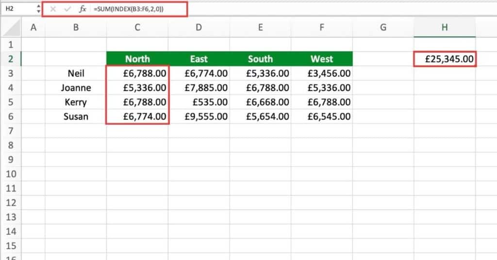
Here’s a breakdown of what’s happening:
- The INDEX function is being used to return a reference to a specific row of data (in this case, row 2) within the range of cells B3:F6.
- The second argument of the INDEX function is set to 0, which means that the function returns a reference to an entire row of data rather than just a single cell.
- The resulting range of cells returned by the INDEX function is then passed as an argument to the SUM function, which adds up the values in that range of cells.
- The final result is the sum of all the values in the second row of the B3:F6 range.
This formula is useful when you want to add up a specific row or column of data within a larger table, without having to manually select all of the cells in that row or column.
INDEX Function Notes
- If the row_num or column_num argument is omitted, the INDEX function returns the entire row or column.
- The INDEX function can be used in combination with other functions such as MATCH to search for a specific value in a table.
- The INDEX function can be used to create dynamic ranges. That adjust automatically when new data is added or removed from a table.