Excel MATCH Function is a powerful and versatile tool used to search for a specific value in a range of cells and return its relative position. It is widely used in many different scenarios, from basic data management to complex calculations, making it a valuable tool for both beginners and advanced Excel users.
Excel MATCH Function Summary
The Excel MATCH function is a powerful tool for locating the position of a lookup value in a row, column, or table. With support for both approximate and exact matching, as well as the use of wildcards for partial matches, this function is highly versatile. When used in combination with the INDEX function, MATCH can be used to easily retrieve a value at a matched position.
MATCH Function Purpose
The purpose of the Excel MATCH Function is to find a specific value in a range of cells and return its relative position. It can be used to look up values in tables, index and match, and perform other complex calculations.
MATCH Function Arguments
The MATCH Function requires three arguments:
- Lookup_value: The value to search for in the range of cells.
- Lookup_array: The range of cells to search in.
- Match_type: Specifies the type of match to be performed. This can be either 1, 0, or -1.
MATCH Function Return Value
The Excel MATCH Function returns the relative position of the lookup value in the lookup array.
MATCH Function Syntax
=MATCH(lookup_value,lookup_array,match_type)Match type information
The Match type is an optional argument in the Excel MATCH function. If the match_type argument is not provided, it defaults to 1, which searches for an exact or next smallest match. When match_type is set to 1 or -1, it is considered an “approximate match”. It’s important to note that the MATCH function will always try to perform an exact match whenever possible, as indicated in the table below:
| Match_type Value | Meaning |
|---|---|
| 1 | Finds the largest value less than or equal to the lookup_value (default) |
| 0 | Finds the first value exactly equal to the lookup_value |
| -1 | Finds the smallest value greater than or equal to the lookup_value and assumes the data is sorted in descending order |
To avoid incorrect results, it’s important to set the match_type to 0 when you need an exact match using the MATCH function in Excel. The default setting of 1 for match_type may give results that appear correct but are actually inaccurate. By explicitly setting a value for match_type, you can ensure that the function behaves as expected and returns accurate results.
Excel MATCH Function Examples
The MATCH function in Excel is used to find the position of a lookup value within a row, column, or table. It supports both approximate and exact matching, and can even handle partial matches using wildcards. Here are some examples of how to use the MATCH function in Excel:
Finding the position of a specific value in a range
This example shows how to use the MATCH function to find the position of a specific value in a range.
Here’s the formula:
=MATCH("apple", A2:A5, 0)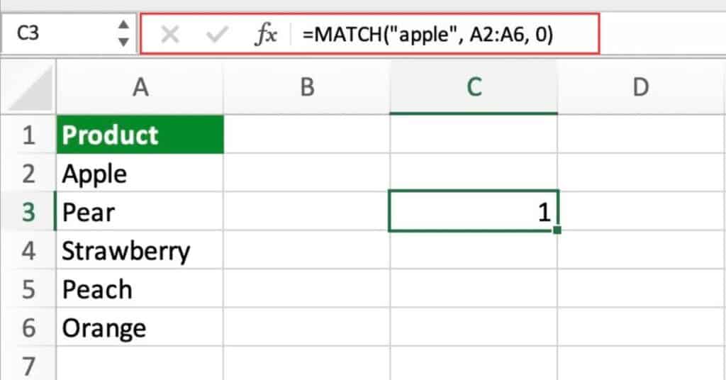
In this example, the MATCH function is used to find the position of the value “apple” in the range A1:A5. The last argument, 0, specifies that an exact match is required.
Finding the closest match in a range
This example shows how to use the MATCH function to find the closest match to a given value in a range.
For this you will need the following formula:
=MATCH(4, A2:A5, 1)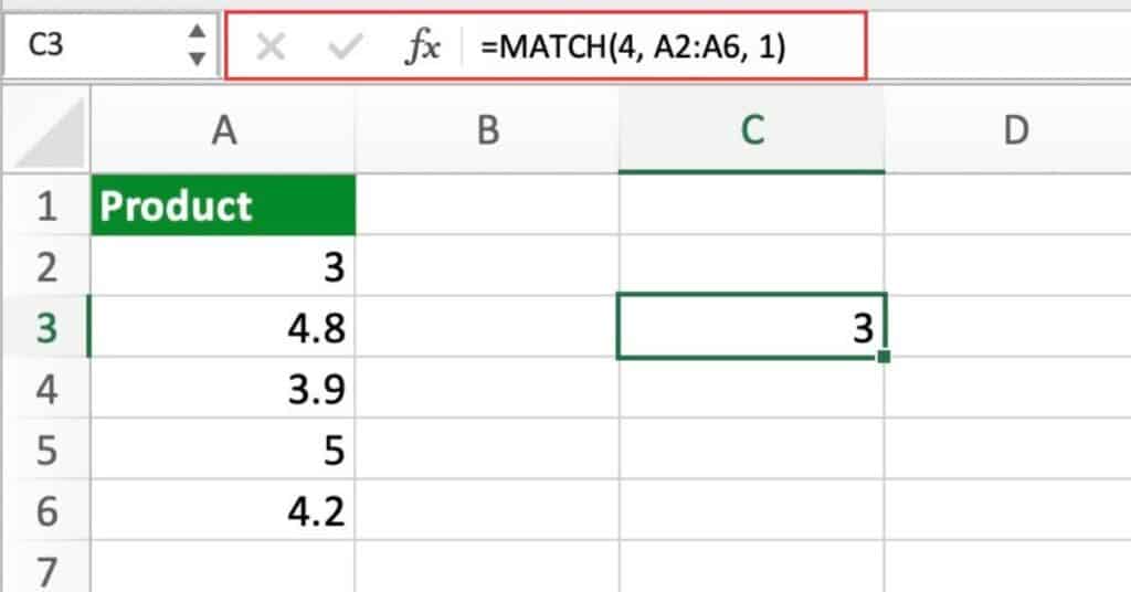
In this example, the MATCH function is used to find the position of the closest match to the value 4 in the range A2:A5. The second argument, A2:A5, specifies the range to search in, and the third argument, 1, specifies that an approximate match is allowed.
Finding the position of the largest value in a range
This example shows how to use the MATCH function to find the position of the largest value in a range.
For this you will need the following formula:
=MATCH(MAX(A2:A6), A2:A6, 0)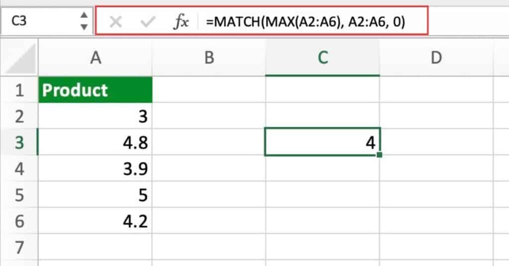
In this example, the MATCH function is used to find the position of the largest value in the range A2:A6. The first argument, MAX(A2:A6), returns the largest value in the range, which is then used as the lookup value. The third argument, 0, specifies that an exact match is required.
Finding the position of the first value that exceeds a threshold
This example shows how to use the MATCH function to find the position of the first value in a range that exceeds a given threshold.
For this you will need the following formula:
=MATCH(TRUE, A2:A6>10, 0)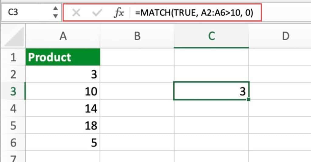
In this example, the MATCH function is used to find the position of the first value in the range A2:A6 that exceeds the threshold of 10. The second argument, A2:A6>10, creates an array of TRUE/FALSE values indicating which elements of the range exceed the threshold.
The MATCH function then returns the position of the first TRUE value in the array, which corresponds to the first element that exceeds the threshold. The third argument, 0, specifies that an exact match is required.
Using a Wildcard with MATCH Function to Find Partial Matches
The MATCH function in Excel can be used to find the position of a value in a range. However, what if you need to find a partial match, such as searching for all names that contain a certain string of characters? This is where a wildcard can be useful.
Suppose you have a list of names in column A, and you want to find the position of the first name that contains the string “mar” (case-insensitive). You can use the wildcard character “*” to represent any number of characters before or after the string “mar”.
Here’s the formula:
=MATCH("mar*",A:A,0)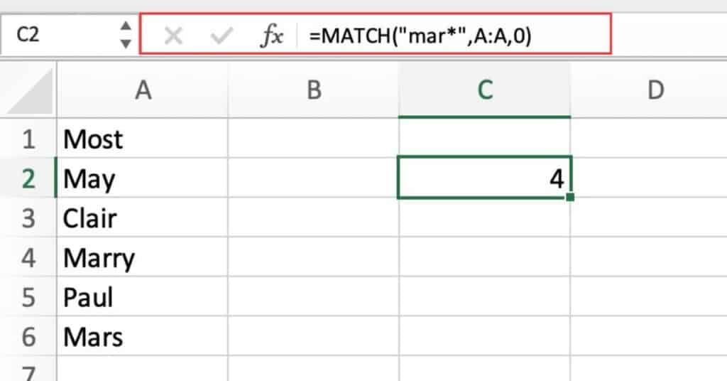
This formula will return the position of the first name that contains the string “mar”, regardless of where it appears within the name.
The first argument, “mar”, is the lookup value that includes the wildcard character “*” before and after the string “mar”.
The second argument, A:A, is the range to search for the lookup value.
The third argument, 0, specifies an exact match (i.e., only returns the position if the lookup value appears exactly in a cell in the range).
Multiple Criteria Match Function
Sometimes you need to match data based on multiple criteria. In this example, we’ll use the MATCH function in combination with other functions. To match data based on two criteria: product and month.
Suppose we have a sales data table that has a list of Products and Month Sales.
We want to find the sales for “Oranges” in “Feb”.
Here’s the formula we can use:
=MATCH(1, (A2:A10="Oranges")*(B2:B10="Feb"), 0)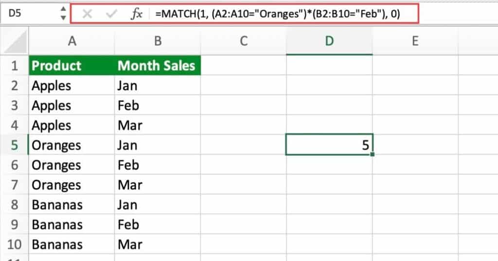
This formula uses the logical operators * (multiplication) and = to check whether each row matches both criteria. The result is an array of TRUE/FALSE values, which is used as the lookup array in the MATCH function. The match_type is set to 0 to get an exact match.
The formula returns 5, which is the row number of the first matching row.
Note that this formula can also be used with other functions. Like INDEX and OFFSET to extract data based on multiple criteria.
Excel MATCH Function Notes
- The MATCH Function can be used in combination with other Excel functions such as INDEX, IF, and SUM to perform complex calculations.
- Match_type 1 performs an approximate match, match_type 0 performs an exact match, and match_type -1 performs an approximate match in descending order.
