Excel’s functions can save you a lot of time and effort. In this article, we’ll look at 10 of the most commonly used Excel functions and explain how they work.
By the end of this article, you’ll have a better understanding of these essential Excel functions and be able to use them to improve your productivity and data analysis skills.
SUM
The SUM function in Excel adds up a range of values in a worksheet.
It can be used to calculate the total of a series of numbers quickly, and it can also be used with other functions and formulas to perform more complex calculations.
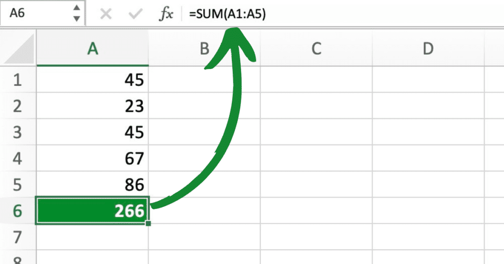
Let’s say you have a column of numbers in cells A1 to A5 that you want to add up.
To do this, you can simply type “=SUM(A1:A5)” into a cell, and the sum of the values in those cells will be calculated and displayed in the cell where you entered the formula.
AVERAGE
The AVERAGE function in Excel calculates the average of a range of numbers.
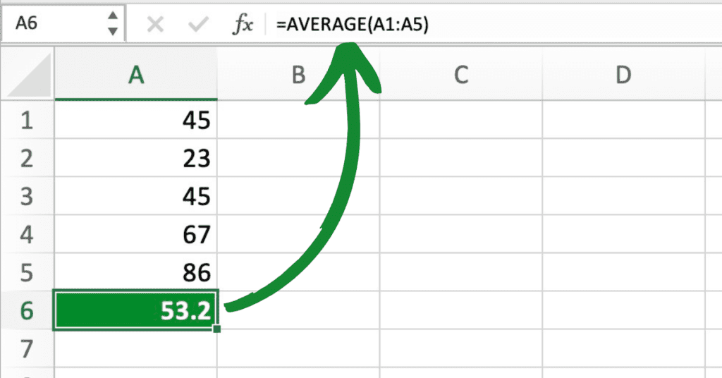
For example, let’s say you have a column of numbers in cells A1 to A5 that you want to average.
To do this, you can type “=AVERAGE(A1:A5)” into a cell, and the average of the values in those cells will be calculated and displayed in the cell where you entered the formula.
COUNT
The COUNT function in Excel counts the number of cells in a range that contain numbers.
For example, let’s say you have a column of numbers in cells A1 to A5, but some of those cells are blank. To count the number of cells in that range that contain numbers, you can type “=COUNT(A1:A5)” into a cell, and the number of cells in that range that contain numbers will be calculated and displayed in the cell where you entered the formula.

As you can see the values in cells A1 to A5 are 2, 4, “”, 8, and 10, respectively, as we can see the formula “=COUNT(A1:A5)” returns a result of 4, which is the number of cells in that range that contain numbers.
MAX
The MAX function in Excel returns the highest value in a range of numbers.
For example, let’s say you have a column of numbers in cells A1 to A5, and you want to find the highest value in that range.
To do this, you can type “=MAX(A1:A5)” into a cell, and the highest value in those cells will be calculated and displayed in the cell where you entered the formula.
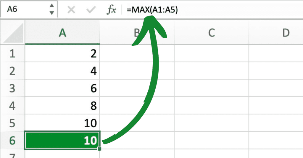
As you can see we have values in cells A1 to A5 are 2, 4, 6, 8, and 10, respectively, and the formula “=MAX(A1:A5)” returns a result of 10, which is the highest value in that range.
MIN
The MIN function in Excel returns the lowest value in a range of numbers.
For example, let’s say you have a column of numbers in cells A1 to A5, and you want to find the lowest value in that range. To do this, you can type “=MIN(A1:A5)” into a cell, and the lowest value in those cells will be calculated and displayed in the cell where you entered the formula.

As you can see we have values in cells A1 to A5 are 2, 4, 6, 8, and 10, respectively, and the formula “=MIN(A1:A5)” returns a result of 2, which is the lowest value in that range.
SUMIF
The SUMIF function in Excel allows you to sum up values in a range of cells that meet specific criteria.
To use the SUMIF function, you need to specify the range of cells you want to evaluate, the criteria you want to use to determine which cells to add up, and the range of cells containing the values you want to sum.
For example, let’s say you have a list of sales data in cells A1 to B10, where column A contains the names of salespeople and column B contains their sales figures.
To calculate the total sales for a specific salesperson, you can use the SUMIF function.
Assuming you want to calculate the total sales for the salesperson named “John”, you can type “=SUMIF(A1:A10, “John”, B1:B10)” into a cell, where A1:A10 is the range of cells containing the salesperson names, “John” is the criteria you want to use to select cells, and B1:B10 is the range of cells containing the sales figures.
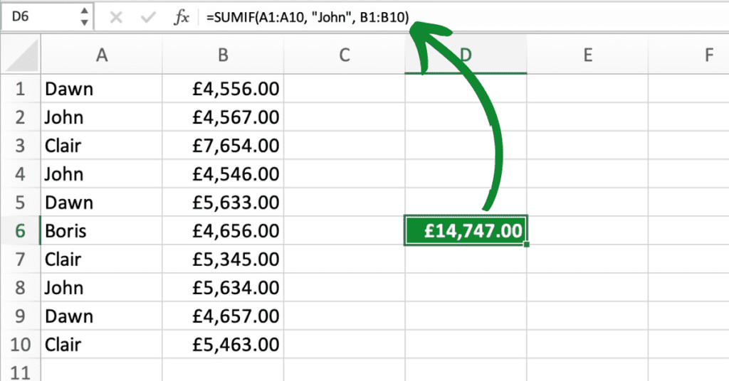
If John’s sales figures are in cells B2, B4, and B8, then the formula “=SUMIF(A1:A10, “John”, B1:B10)” would return a result of the total sales for John, which is the sum of cells B2, B4, and B8.
IF
The IF function in Excel allows you to test a condition and return one value if the condition is true, and another value if the condition is false.
To use the IF function, you need to specify the condition you want to test, and the values you want to return if the condition is true or false.
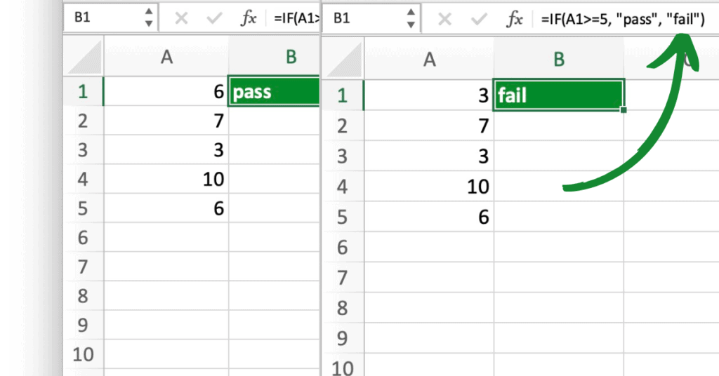
For example, let’s say you have a column of numbers in cells A1 to A5, and you want to label each value as either “pass” or “fail” based on whether it is greater than or equal to 5.
To do this, you can type “=IF(A1>=5, “pass”, “fail”)” into cell B1, and the formula will check if the value in cell A1 is greater than or equal to 5.
If it is, the formula will return “pass”, and if it is not, the formula will return “fail”.
If the value in cell A1 is 6, then the formula “=IF(A1>=5, “pass”, “fail”)” would return a result of “pass”, because 6 is greater than or equal to 5.
VLOOKUP
The VLOOKUP function in Excel allows you to search for a specific value in a table of data, and return a related value from the same row.
To use the VLOOKUP function, you need to specify the value you want to look up, the table of data you want to search in, the column of data that contains the corresponding value you want to return, and whether you want an exact match or an approximate match.
For example, let’s say you have a table of employee information, including their names, employee IDs, and salaries.
To find the salary of a specific employee based on their Name, you can use the VLOOKUP function.
Assuming the table is in cells A1 to C5, you can type “=VLOOKUP(“101″Boris”, A1:C5, 3, FALSE)” into a cell, where Boris is the employee name you want to search for, A1:C5 is the range of cells containing the employee information, 3 is the column containing the salary information, and FALSE means you want an exact match.
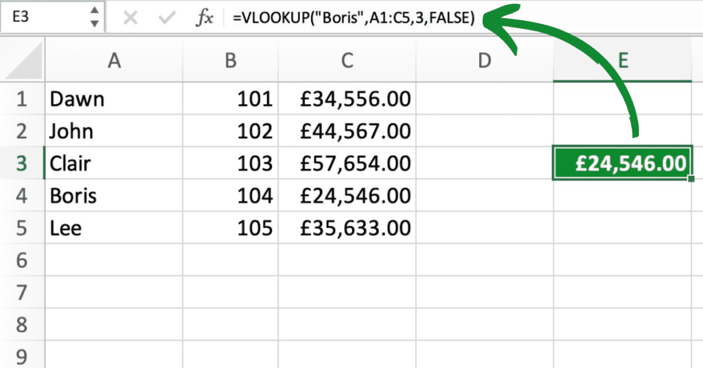
If the employee with the name Boris has a salary of £24,546.00, then the formula “=VLOOKUP(“Boris”, A1:C5, 3, FALSE)” would return a result of £24,546.00.
CONCATENATE
The CONCATENATE function in Excel allows you to join together two or more text strings into a single string.
To use the CONCATENATE function, you need to specify the text strings you want to join together and separate them with commas.
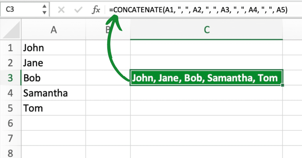
For example, let’s say you have a list of names in cells A1 to A5, and you want to create a single string that includes all of the names separated by commas.
To do this, you can type “=CONCATENATE(A1, “, “, A2, “, “, A3, “, “, A4, “, “, A5)” into a cell, and the formula will join together all of the names with commas and a space between each name.
If the names in cells A1 to A5 are “John”, “Jane”, “Bob”, “Samantha”, and “Tom”, respectively, then the formula “=CONCATENATE(A1, “, “, A2, “, “, A3, “, “, A4, “, “, A5)” would return a result of “John, Jane, Bob, Samantha, Tom”.
ROUND
The ROUND function in Excel allows you to round a number to a specific number of decimal places.
To use the ROUND function, you need to specify the number you want to round, and the number of decimal places you want to round it to.
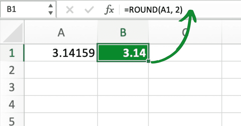
For example, let’s say you have a calculated result in cell A1 that has several decimal places, but you only want to display it with two decimal places. To do this, you can type “=ROUND(A1, 2)” into a cell, and the formula will round the number in cell A1 to two decimal places.
If the number in cell A1 is 3.14159, then the formula “=ROUND(A1, 2)” would return a result of 3.14, which is the original number rounded to two decimal places.
This guide is to help with the Most Commonly Used Excel Functions. Yet, if you want to learn more head over to my basic excel page. This is the perfect place to learn whether you are a beginner to excel or an expert there is something to learn.
Or even discover even more Excel functions in our dedicated section.
If you prefer to watch excel demonstrations then I have put together a YouTube channel that is well worth checking out if a video is your thing.
