The Excel OFFSET function is a powerful tool that allows users to dynamically reference a range of cells in a worksheet. This function is useful for situations where data needs to be updated regularly, and the range of cells that need to be referenced changes. By using the OFFSET function, users can avoid the tedious task of updating cell references manually, saving time and reducing the risk of errors.
Excel OFFSET Function Summary
The OFFSET function in Excel is a powerful tool for manipulating data ranges. By returning a reference to a cell or a range of cells that is offset from a given reference, OFFSET enables you to create dynamic ranges that can adjust to changes in data. Learn how to use OFFSET to streamline your Excel workflow and boost your productivity.
OFFSET Function Purpose
The main purpose of the Excel OFFSET function is to return a reference to a range of cells that is a specified number of rows and columns from a starting cell. This can be useful in a wide range of scenarios, such as creating dynamic charts, analyzing data, and creating reports.
OFFSET Function Arguments
The OFFSET function requires five arguments:
- reference: the starting cell for the range
- rows: the number of rows to move down from the starting cell
- columns: the number of columns to move right from the starting cell
- height: the number of rows in the range to be returned
- width: the number of columns in the range to be returned
OFFSET Function Return value
The OFFSET function returns a reference to a range of cells, which can be used in other functions and formulas in the worksheet.
OFFSET Function Syntax
=OFFSET(reference, rows, columns, [height], [width])OFFSET Function Examples
we’re going to explore the OFFSET function in Excel and demonstrate how it can be used in practical scenarios. Whether you’re working with large datasets or need to create dynamic charts and tables, OFFSET can be a powerful tool to help you achieve your goals. By the end of this post, you’ll have a solid understanding of how the OFFSET function works and how it can be used to streamline your Excel workflow. Let’s dive in!
Using the OFFSET Function to Retrieve Data from a Range
The OFFSET function can be used to retrieve data from a range by specifying the number of rows and columns to offset from a starting cell. This example demonstrates how the OFFSET function can be used to retrieve data from a range by offsetting a starting cell by three rows and one column.
So lets add the following function to our spreadsheet:
=OFFSET(A1,3,4)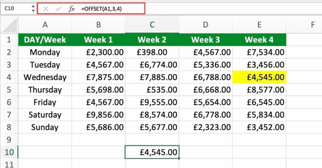
Here’s what’s happening with the formula:
- In the formula the starting point is cell A1.
- The rows argument is 3, which means we want to move down three rows from cell A1.
- The columns argument is 4, which means we want to move four columns to the right from cell A1.
- Therefore, the OFFSET function returns a reference to the cell that is three rows down and four column to the right of cell A1, which is cell E4.
If the value in cell E4 changes, the OFFSET function will automatically update to return the value of the cell that is three rows down and four columns to the right of the new value in cell E4.
Extracting Data for a Specific Day Across Multiple Weeks
Suppose we want to extract the earnings for Wednesday across all weeks using the previous example.
To accomplish this, we can use the formula:
=OFFSET(A1,3,1,1,4)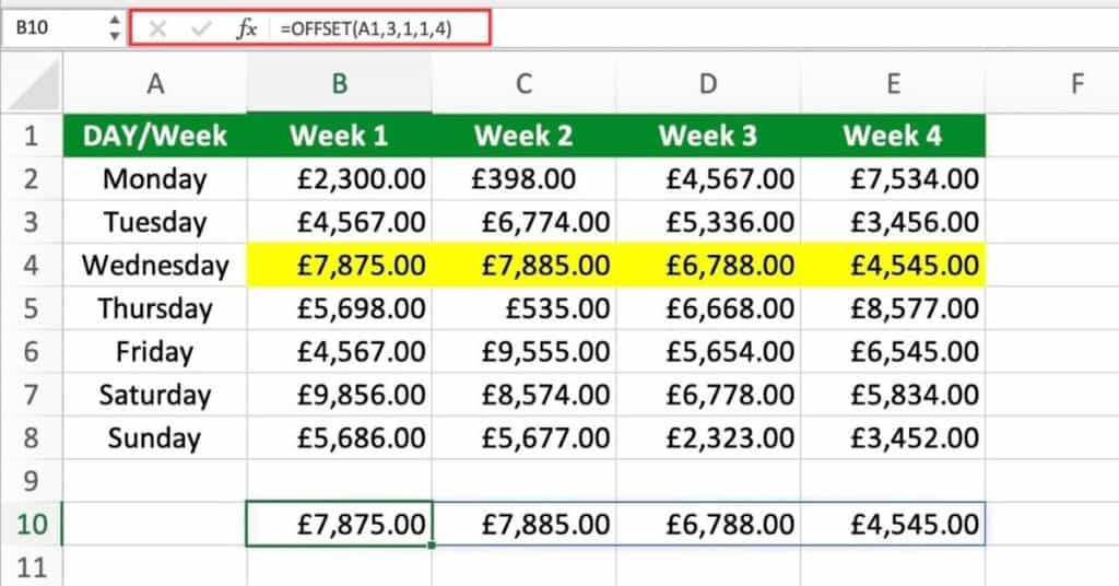
Here’s what’s happening with the formula:
- A1: This is the starting cell from which we want to offset. In this case, it’s the cell containing the first earnings value.
- 3: This represents the number of rows we want to offset from the starting cell. Since we want to retrieve data for Wednesday, which is three rows down from the starting cell, we specify 3.
- 1: This represents the number of columns we want to offset from the starting cell. Since Wednesday’s earnings are one column to the right of the starting cell, we specify 1.
- 1: This represents the number of rows we want to retrieve from the offset cell. Since we only want to retrieve one row (Wednesday’s earnings for a single week), we specify 1.
- 4: This represents the number of columns we want to retrieve from the offset cell. Since we want to retrieve earnings data for all days of the week, we specify 4 (one column for each day).
By entering this formula as an array formula and dragging it down to subsequent rows, we can retrieve earnings data for Thursday across multiple weeks.
Using the OFFSET Function to Sum a Range
When working with large datasets in Excel, it can be useful to have a quick way to summarize or analyze certain sections of the data. The SUM function, in combination with the OFFSET function, provides a powerful tool for doing just that.
By using OFFSET to define a specific range of cells. We can easily sum the values in that range with the SUM function. In this section, we’ll explore how to use the SUM and OFFSET functions together. To perform quick and effective data analysis in Excel.
So, working with the same data set as before. We will use the OFFSET function to define a range of cells to be summed by the SUM function
=SUM(OFFSET(A1,1,2,7,1))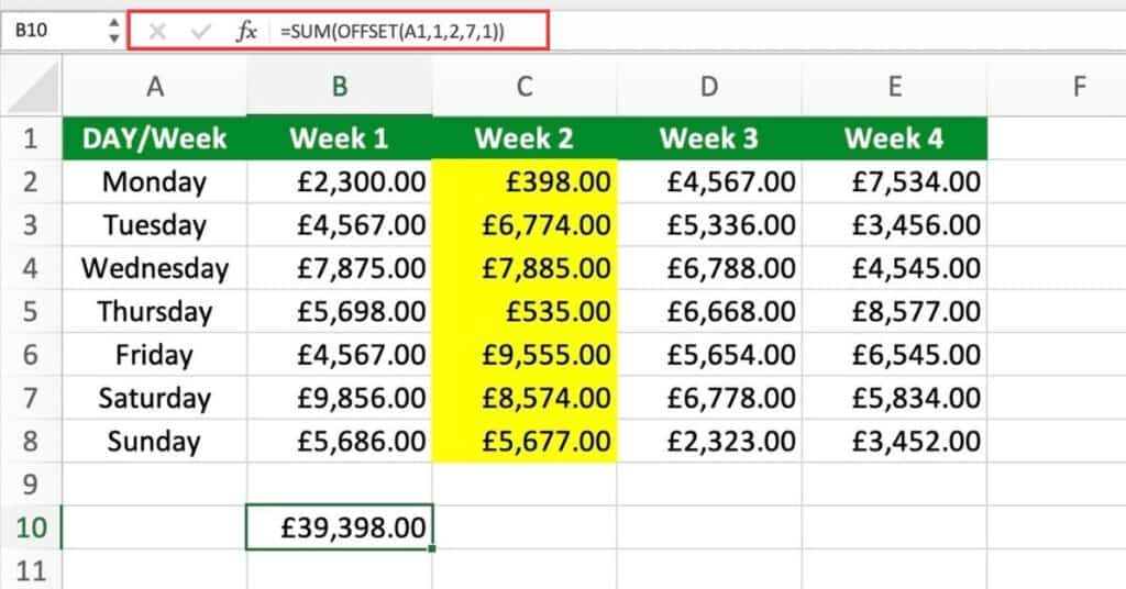
Here’s what’s happening with the formula:
- The starting cell is A1.
- The arguments “1” and “2” mean that we want to offset the starting cell by 1 row and 2 columns, so the starting cell becomes C2.
- The arguments “7” and “1” define a range of 7 rows and 1 column, so we end up with the range C2:C8.
- The SUM function then sums the values in that range.
In other words, the formula is summing the values in the range C2:C8. Which is offset from the starting cell A1 by 1 row and 2 columns.
OFFSET Function Notes
- Be careful when using the OFFSET function, as it can slow down worksheet performance when used excessively.
- Use the absolute reference ($ sign) to lock the starting cell of the OFFSET function, if necessary.
- It is important to ensure that the specified range is within the boundaries of the worksheet to avoid errors.