Calculating ratios is an essential skill in Excel, and it’s crucial to know how to do it quickly and efficiently. In this blog post, we will learn how to calculate the ratio between two numbers using the division formula in Excel.
How to Quickly Calculate Ratio in Excel
Step-by-Step Guide to Calculate Ratio in Excel:
- First, open a new or existing Excel spreadsheet.
- Enter the two numbers that you want to calculate the ratio for in two adjacent cells.
- Select the cell where you want to display the ratio.
- In that cell, type the equal sign (=) to begin the formula.
- Then, type the cell reference of the numerator (the top number in the ratio).
- Next, type a forward slash (/) to indicate division.
- Now, type the cell reference of the denominator (the bottom number in the ratio).
- Next add &”:”&”1″
- Press Enter to complete the formula, and the ratio will appear in the selected cell.
For example, suppose you want to calculate the ratio of 10 to 5.
In that case, you would enter the numbers in adjacent cells (A1 and B1), select cell C1 where you want to display the ratio, and enter the formula:
=A1/B1&":"&"1"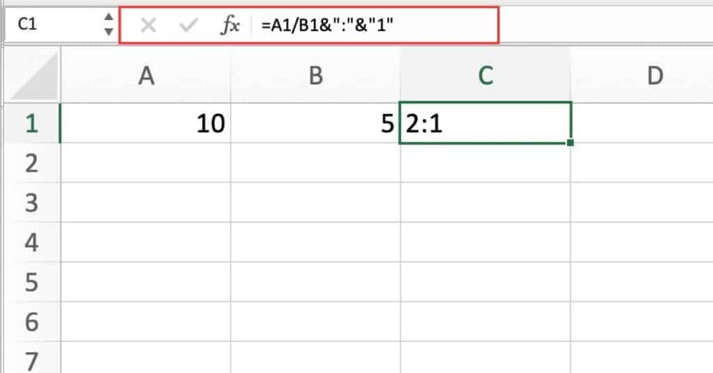
How the Formula Works
This formula takes the value in cell A1 and divides it by the value in cell B1, then concatenates the result with a colon and the number 1.
So our example, if cell A1 contains the value 10 and cell B1 contains the value 5, the formula would return the value 2:1.
Things to Keep in Mind
- Make sure that the numerator and denominator are in the correct cells.
- Use absolute cell references (with dollar signs) if you plan to copy and paste the formula to other cells.
- If the denominator is zero, the result will be an error (#DIV/0!).
- In conclusion, calculating ratios in Excel is a straightforward process that involves using the division formula. By following the steps above, you can quickly and efficiently calculate ratios in your spreadsheets.
GCD Function to Calculate Ratio in Excel
The Greatest Common Divisor (GCD) function in Excel is an incredibly useful tool for calculating the ratio between two numbers. This is especially helpful when dealing with fractions, as the GCD allows you to reduce the fraction to its lowest terms. In this blog, we will show you how to use the GCD function to calculate a ratio in Excel.
First, let’s start with a simple example. Let’s say you have two numbers, A1 and B1, and you want to calculate the ratio between them. To do this, you can use the GCD function in Excel. The formula looks like this:
=A1/GCD(A1,B1)&":"&B1/GCD(A1,B1)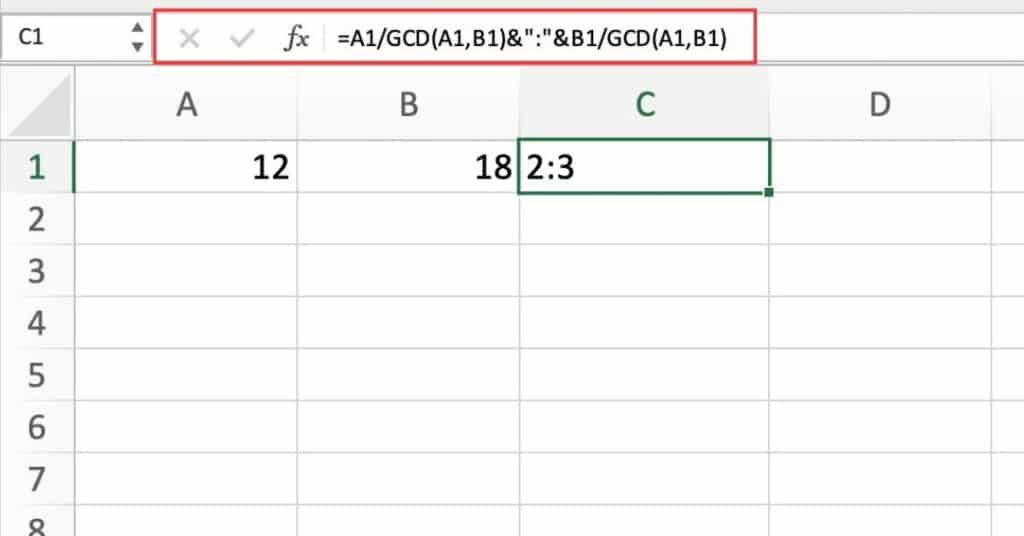
Let’s break this down.
The GCD function takes two numbers as arguments, A1 and B1.
It then finds the greatest common divisor of these two numbers.
In our example, let’s say A1 = 12 and B1 = 18.
The GCD of these two numbers is 6. The formula then takes the first number (A1) and divides it by the GCD (6).
This gives us 12/6 = 2.
The formula then takes the second number (B1) and divides it by the GCD (6).
This gives us 18/6 = 3. These two numbers are then combined into a ratio, 2:3.
So, using the GCD function in Excel, you can quickly and easily calculate the ratio between two numbers.
This is especially useful for dealing with fractions, as the GCD allows you to reduce the fraction to its lowest terms.
Give it a try and see how easy it is to calculate ratios in Excel!
Using SUBSTITUTE and TEXT for Ratio Calculation
Knowing how to calculate ratios in Excel can be a handy tool for businesses, as well as individuals who need to analyze data. Ratios are often used to measure financial performance, compare companies, and look at trends over time. When calculating ratios in Excel, there are a few different formulas you can use.
The SUBSTITUTE and TEXT formulas can be used to calculate ratios in Excel in the following manner:
=SUBSTITUTE(TEXT(A1/B1,"#####/#####"),"/",":")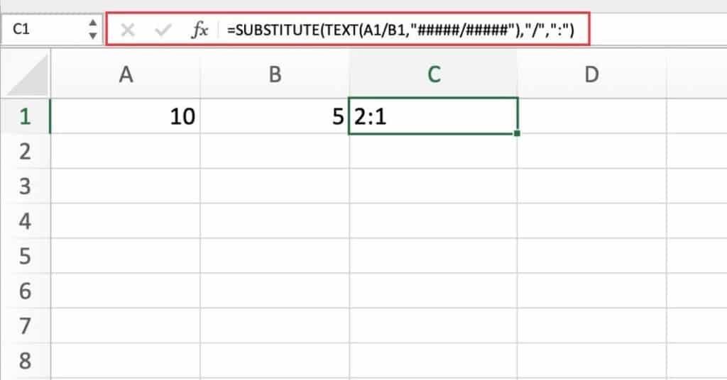
The A1 and B1 cells refer to the two numbers we are using to calculate the ratio.
The SUBSTITUTE and TEXT formulas together convert the result of the ratio calculation into a text string, with the “/” replaced with a “:”.
For example, if cell A1 contained 10 and cell B1 contained 5, then the result of the formula would be “2:1”.
Using the SUBSTITUTE and TEXT formulas to calculate ratios in Excel is a great way to quickly and easily analyze data.
By changing the parameters of the formula, you can easily adjust the type of ratio you are calculating.
We hope this blog was helpful in demonstrating how to calculate ratios in Excel using the SUBSTITUTE and TEXT formulas.
Effortlessly Calculate Ratios with Excel’s ROUND Function
Calculating ratios is a common task in many fields, such as finance, statistics, and engineering. Excel provides several built-in functions to make it easy to calculate ratios, and one of these functions is the ROUND function. The ROUND function can be used to round the result of a calculation to a specified number of decimal places. In this blog, we will demonstrate how to use the ROUND function to calculate a ratio in Excel.
Step 1: Enter the Data
First, we need to enter the data that we want to calculate the ratio for. Let’s assume we have two cells, A1 and B1, that contain the values we want to divide to calculate the ratio.
In this example, we will use 10 and 3 as the values.
Step 2: Write the Formula
To calculate the ratio, we need to divide the value in cell A1 by the value in cell B1. We can do this using the division operator “/”. The formula to do this is:
=A1/B1This formula will give us the ratio as a decimal value. However, we want to round the result to one decimal place and display it in a specific format. To do this, we will use the ROUND function and concatenate the result with a colon (“:”) and a denominator of 1. The formula to do this is:
=ROUND(A1/B1,1)&":"&1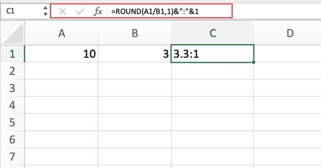
Let’s break down this formula step by step.
The first part of the formula, ROUND(A1/B1,1), calculates the ratio as a decimal value and rounds it to one decimal place.
The second argument of the ROUND function, 1, specifies the number of decimal places to round to.
The second part of the formula, “&”:”&1″, concatenates the result of the first part of the formula with a colon (“:”) and a denominator of 1.
The ampersand “&” symbol is used to concatenate the text strings.
The colon is added to separate the numerator and denominator of the ratio, and the denominator of 1 is added to specify that the denominator is 1.
Step 3: Apply the Formula
To apply the formula, simply enter it into a cell in Excel, and press Enter. The result will be displayed in the cell.
In our example, the result of the formula is “3.3:1”, which means that the value in cell A1 is 3.3 times larger than the value in cell B1.
You should now know How to Quickly Calculate Ratio in Excel depending on the situation you are facing.