Excel VLOOKUP is a powerful function that allows users to search for and retrieve data from a table based on a specific value. The function is used extensively in data analysis and is a popular tool for data manipulation and lookup tasks. VLOOKUP stands for “vertical lookup” because it searches vertically through a table of data to find a match.
Excel VLOOKUP Function Summary
VLOOKUP, short for “Vertical Lookup,” is a powerful Excel function that allows you to retrieve data from a table arranged vertically. It supports both approximate and exact matching, as well as the use of wildcards (*?) for partial matches. As a premade function in Excel, VLOOKUP allows you to quickly search across columns and retrieve the data you need with ease.
VLOOKUP Purpose
The purpose of the Excel VLOOKUP function is to search for a specific value in a table of data and return a corresponding value from a different column in the same row.
VLOOKUP Arguments
- Lookup_value: The value to search for in the first column of the table.
- Table_array: The range of cells that contains the table of data to search.
- Col_index_num: The column number of the value to return from the table, where the first column in the table is 1.
- Range_lookup: A logical value that determines whether an exact or approximate match is required. If TRUE or omitted, an approximate match is returned. If FALSE, an exact match is required.
VLOOKUP Return value
The Excel VLOOKUP function returns a value from a table based on a specific lookup value.
VLOOKUP Syntax
=VLOOKUP(lookup_value, table_array, col_index_num, [range_lookup])Match modes
VLOOKUP is a powerful Excel function that can help you quickly search for a specific value in a large dataset. One of the key features of VLOOKUP is its match mode, which determines how the function searches for the lookup value.
There are three match modes in VLOOKUP:
- Exact Match: This is the default match mode for VLOOKUP. In this mode, VLOOKUP searches for an exact match of the lookup value in the leftmost column of the lookup table.
- Approximate Match (TRUE/FALSE): In this mode. VLOOKUP searches for the closest match of the lookup value in the leftmost column of the lookup table. This mode is useful when you need to search for a value that falls within a range of values, such as when using a lookup table with price ranges or age groups.
- Approximate Match (1/0): This mode is similar to the TRUE/FALSE mode. But instead of using the words TRUE or FALSE, you use the numbers 1 or 0, respectively.
VLOOKUP Examples
Excel’s VLOOKUP function is a powerful tool for finding and retrieving data from tables. In this section, we’ll explore some practical examples of how you can use VLOOKUP. To streamline your data analysis and make your work in Excel more efficient.
Basic VLOOKUP function
Let’s first look at a basic VLOOKUP and we will use it to search for a product in the first column and return the corresponding value in the second column, with an exact match (FALSE) required.
=VLOOKUP("Product A",A2:B7,2,FALSE)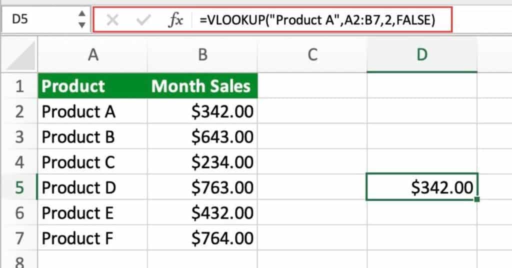
In this example, the VLOOKUP function is used to search for “Product A” in the first column of the table and return the corresponding value from the second column.
Exact Match with VLOOKUP
Suppose we have a table that lists the product names and their corresponding prices, and we want to find the price for a specific product. In this case, we want to use an exact match to ensure that we get the correct price.
We would need the following formula:
=VLOOKUP("Product B", A2:B5, 2, FALSE)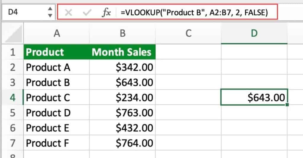
In this formula, we are looking up the price for “Product B” in the range A2:B5. The “2” indicates that we want to return the value from the second column of the table (i.e., the price column), and the “FALSE” indicates that we want an exact match. The formula will return the value “$643”, which is the price for “Product B”.
Approximate Match with VLOOKUP
Suppose we have a table that lists the tax rates for different income levels, and we want to find the tax rate for a specific income. In this case, we want to use an approximate match to find the tax rate for the income bracket that includes the specified income.
We would need the following formula:
=VLOOKUP(B2,E2:F5,2,TRUE)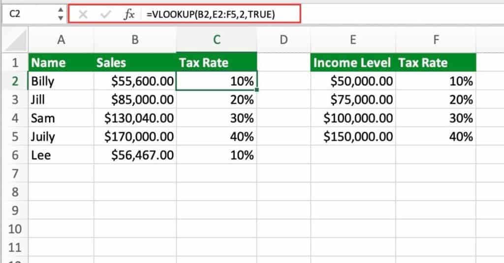
In this formula, we are looking up the tax rate for Billy we first select his salary in cell B2. We now select the table that lists the tax rates for different income levels in E2:F5.
The “2” indicates that we want to return the value from the second column of the table (i.e., the tax rate column) and the “TRUE” indicates that we want an approximate match.
The formula will return the value “10%”, which is the tax rate for the income bracket that includes $50,000.
VLOOKUP is Not Case-insensitive
The Excel VLOOKUP function can perform a case-insensitive lookup. In the following example, the function searches for “BILLY” (cell D2) in the first column of the table regardless of the letter case.
=VLOOKUP(D2,A2:B6,2,FALSE)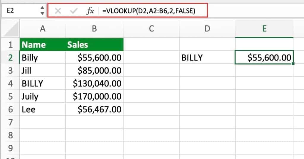
The VLOOKUP function in Excel is not case-sensitive, meaning that it treats uppercase and lowercase letters as the same.
For instance, if the function is used to lookup “BILLY” in a table, it will also match “Billy”, “BilLY”, “billY”, etc. Therefore, the VLOOKUP function will return the first instance of the matched value, regardless of its case.
In cases where a case-sensitive lookup is required. One can use the combination of INDEX, MATCH, and EXACT functions in Excel.
VLOOKUP First Match Only
Suppose you have a table of products and their corresponding prices, and you want to find the price of a specific product. However, there are duplicate entries of the product in the table, and you want to only retrieve the first match. You can use the VLOOKUP function with the IF function to achieve this.
=IF(VLOOKUP("Product A",A2:B6,2,FALSE)<>"",VLOOKUP("Product A",A2:B6,2,FALSE),"Not Found")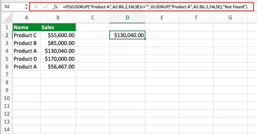
The first VLOOKUP function looks up the value “Product A” in the range A2:B6 and retrieves the value in the 2nd column (i.e., the price) if an exact match is found (indicated by the FALSE argument).
The IF function checks if the result of the first VLOOKUP is not blank, and if it is not, then it returns the result. Otherwise, it returns the text “Not Found”.
VLOOKUP Wildcard Match
Suppose you have a table of products and their corresponding prices, and you want to find the price of a specific product, but you only remember a part of the product name. You can use the VLOOKUP function with the wildcard character * to achieve this.
=VLOOKUP("*Prod*",A2:B6,2,FALSE)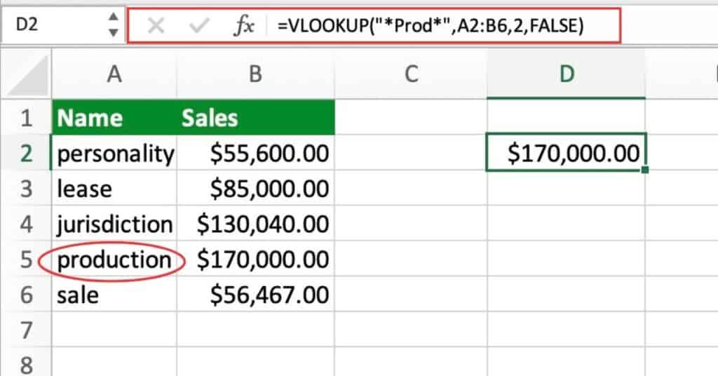
The VLOOKUP function looks up the value “Prod” in the range A2:B6 and retrieves the value in the 2nd column (i.e., the price) if an exact match is found (indicated by the FALSE argument). The * character acts as a wildcard, allowing for partial matches.
Two-Way Lookup
Suppose you have a table with multiple rows and columns, and you want to retrieve a value that intersects a specific row and column. You can use the VLOOKUP function in combination with the INDEX and MATCH functions to achieve this.
=INDEX(B2:E6,MATCH("Product B",A2:A6,0),MATCH("Quarter 3",B1:E1,0))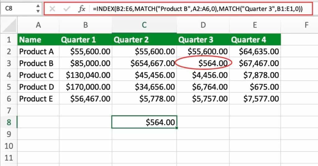
The first MATCH function looks up the value “Product B” in the range A2:A6 and returns the position of the match in the array.
The second MATCH function looks up the value “Quarter 3” in the range B1:E1 and returns the position of the match in the array.
The INDEX function takes the range B2:E6 and retrieves the value at the intersection of the row and column determined by the two MATCH functions.
Multiple Criteria
Suppose you have a table with sales data, including the product, the month, and the sales amount. You want to retrieve the sales amount for a specific product and month. You can use the VLOOKUP function with multiple criteria to do this.
We would need the following formula:
=VLOOKUP(A1&B1,$A$2:$C$10,3,FALSE)This formula concatenates the values in cells A1 and B1 using the “&” symbol, creating a combined lookup value. The formula then looks up the combined value in the first two columns of the table ($A$2:$B$10). Then returns the sales amount from the third column.
VLOOKUP Handling #N/A Errors
Sometimes, when you use the VLOOKUP function, you may encounter #N/A errors if the lookup value is not found in the table. Here’s an example of how to handle this error:
- Assume that you have a table of employee data, including the employee ID, name, department, and salary.
- You want to retrieve the salary of a specific employee, but the employee may not be in the table. To handle the #N/A error, you can use the IFERROR function, like this:
=IFERROR(VLOOKUP(E6,$A$2:$C$9,3,FALSE),"Employee not found")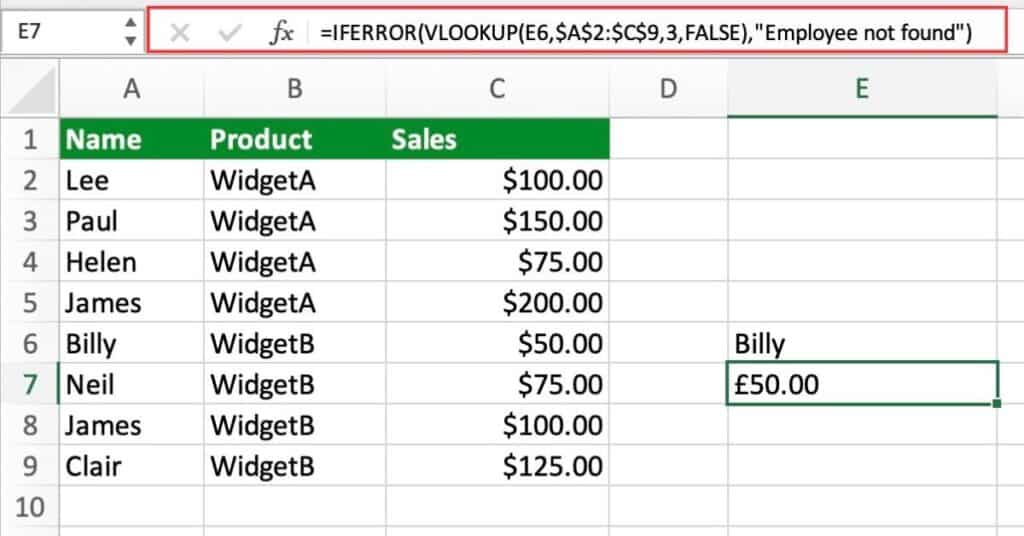
This formula uses the VLOOKUP function to look up the employee name in the first column of the table ($A$2:$D$10). The employee name is in cell E6 and returns the corresponding salary from the third column. If the name is not found, the IFERROR function returns the text “Employee not found” instead of the #N/A error.
Common Errors in VLOOKUP Function
- N/A error: Occurs when the lookup value is not found in the table array or the table array is not sorted in ascending order.
- #REF! error: Occurs when the range_lookup argument is set to an invalid value or the table array reference is incorrect.
- #VALUE! error: Occurs when the lookup value or the column index number is not valid.
- #NAME? error: Occurs when the VLOOKUP function is misspelled or not recognized as a valid function in Excel.
- Incorrect range size error: Occurs when the range specified in the table_array argument has more than one column but the column index number is set to 1.
- Duplicates in the lookup column: If there are duplicates in the lookup column. VLOOKUP will only return the first match, and subsequent matches will be ignored.
- Not using exact match: If the range_lookup argument is set to TRUE (approximate match). VLOOKUP may return unexpected results or the wrong value.
These errors can be resolved by carefully checking the inputs and ensuring that the correct arguments are used in the function.
VLOOKUP Notes
- VLOOKUP function can only search for a value in the first column of a table. Then return a corresponding value from another column in the same row.
- If the lookup value is not found in the first column of the table, the function will return an #N/A error.
- It is important to ensure that the table is sorted in ascending order by the column used for lookup value in order to get correct results.
Alternatives to VLOOKUP in Excel
When it comes to looking up and retrieving data from a table in Excel. VLOOKUP is one of the most commonly used functions. However, there are several alternatives to VLOOKUP. That can be used depending on the specific needs and requirements of your data.
Here are some alternatives to VLOOKUP:
- INDEX/MATCH: The INDEX/MATCH function is a powerful alternative to VLOOKUP that is more flexible and versatile. It allows you to search for a value in a table and return a value in the same row. Without any limitations on the position of the lookup value.
- XLOOKUP: The XLOOKUP function is a newer function that is designed to replace VLOOKUP and HLOOKUP. It allows you to search for a value in a table and return a value in the same row or column with support for fuzzy matching and array inputs.
- SUMIFS: The SUMIFS function can be used as an alternative to VLOOKUP. When you need to retrieve a sum of values that meet multiple criteria. It allows you to sum values in a range based on one or more conditions.
- IFERROR: The IFERROR function is not a direct replacement for VLOOKUP. But it can be used to handle errors that may occur when using VLOOKUP. It allows you to specify a value or formula to return if an error occurs. Which can be useful in avoiding #N/A errors in your spreadsheet.
Overall, there are several alternatives to VLOOKUP that can be used in Excel. Depending on your specific needs and data requirements. It’s important to understand the strengths and limitations of each function. To determine which one is the best fit for your particular situation.