What is a Range in Excel? (Complete Tutorial)

Excel is versatile and crucial for managing finances and creating business reports. Understanding What is a Range in Excel is essential for working with data effectively. In this blog, we’ll provide a complete tutorial on what ranges are in Excel, how to use them, and apply various operations.

Introduction

A brief explanation of what a Range is in Excel

In Microsoft Excel, a range refers to a group of cells that are selected together to perform a specific action or function.

A range can include a single cell, a group of adjacent cells, multiple rows or columns, or even non-contiguous cells that are not next to each other.

By selecting a range of cells, you can perform various operations on them at once, such as formatting, entering data, or applying formulas.

Ranges can also be named, which makes them easier to reference in formulas and macros.

Understanding how to work with ranges is an essential skill for using Excel effectively.

Importance of understanding Range in Excel

Understanding the range in Microsoft Excel is crucial for efficient data management and analysis.

Here are some reasons why:

• Data organization: Ranges group cells for easy data organization and management, enabling formatting, sorting, filtering, and calculation within the specified area without affecting other cells.

• Speed and efficiency: Selecting a range of cells is faster than individual cells and allows for efficient actions like copying, pasting, and formatting with minimal clicks.

• Accurate calculations: Using cell ranges in formulas and functions increases calculation precision by accurately including designated cells and reducing the risk of errors.

• Improved analysis: Ranges expedite analysis and comparison of large datasets. Range references facilitate chart creation, pivot tables, and other visualizations to identify trends and patterns.

• Automation: Mastery of ranges is crucial when automating Excel tasks and creating macros. VBA code often references ranges, streamlining data manipulation through programming.

Omit, understanding the range in Excel is essential for efficient and accurate data management, analysis, and automation.

It enables you to work more quickly and accurately, saving time and improving productivity.

Types of Ranges in Excel

Cell Ranges

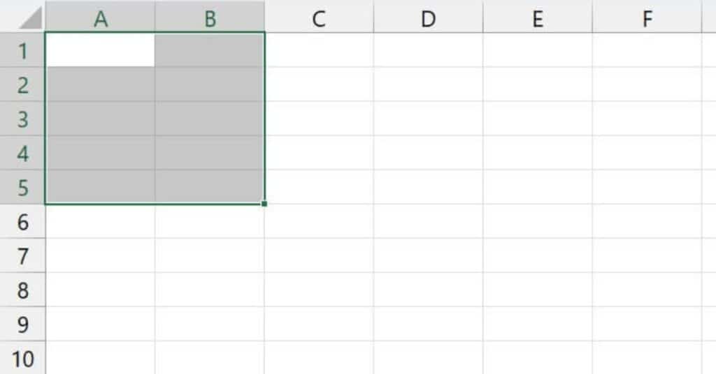
Excel cell range is a group of adjacent cells selected to perform operations like data entry, formatting, and calculation.

Defined by upper-left and lower-right corners separated by a colon.

e.g. A1:B5 encompasses all cells between A1 and B5, including columns A and B and rows 1 to 5.

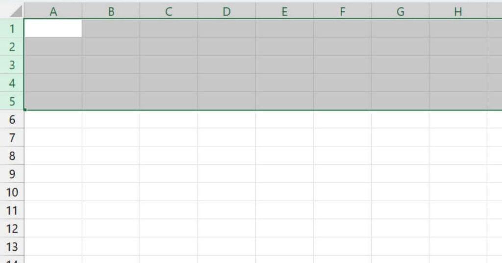
Row Ranges

Excel row range is a group of adjacent rows selected. Defined by the top and bottom row numbers separated by a colon, e.g., 1:5 encompasses all rows between row 1 and row 5, including all columns in those rows.

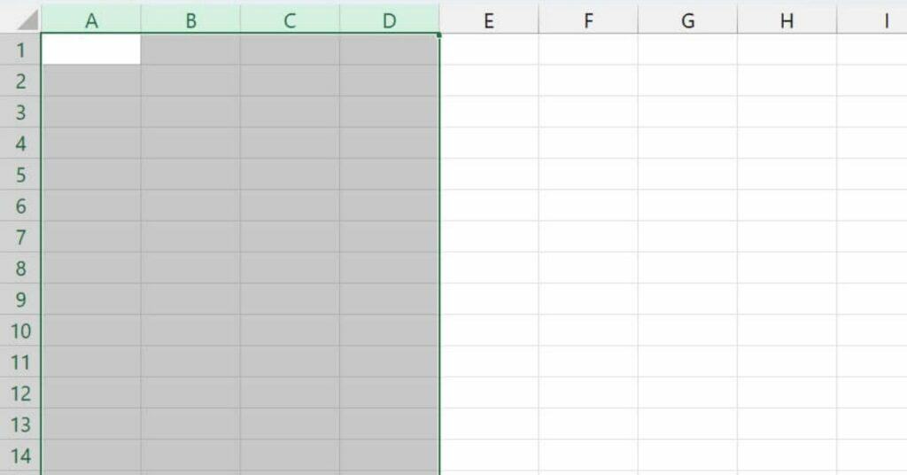
Column Ranges

Excel column range is a group of adjacent columns selected. Defined by the left and right column letters separated by a colon, e.g., A:D encompasses all columns between column A and column D, including all rows in those columns.

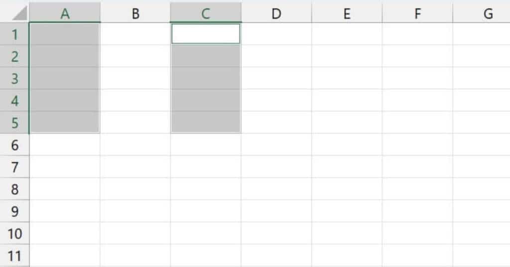
Non-contiguous Ranges

Non-contiguous ranges in Microsoft Excel refer to multiple ranges of cells that are not next to each other but are selected together to perform a specific operation.

This means that the selected cells are not connected in a single continuous range.

For example, you might select cells A1:A5 and C1:C5 to create a non-contiguous range that includes two separate ranges of cells.

You can select non-contiguous ranges using the keyboard or mouse.

I will cover how to select a range below.

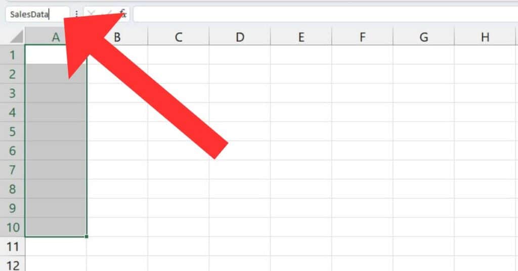
Named Ranges

Named ranges in Microsoft Excel are a way to assign a name to a specific range of cells in a worksheet.

This makes it easier to refer to that range of cells in formulas, functions, and other operations, rather than using the cell references.

For example, you might name the range A1:A10 as “SalesData” to make it easier to refer to that range in formulas or other operations.

More on named Ranges below.

How to Select a Range in Excel

Using the Mouse

Selecting a range of cells in Excel using the mouse is a quick and easy way to highlight a group of cells you want to work with.

To select a range of cells using the mouse in Excel, follow these steps:

1. Click on the cell in the upper left corner of the range you want to select.
2. Press and hold down the left mouse button.
3. Drag the mouse pointer to the lower right corner of the range you want to select.
4. Release the mouse button.

The selected range of cells will be highlighted in blue.

Selecting a non-contiguous range

If you want to select a non-contiguous range of cells (i.e. cells that are not adjacent to each other), follow these steps instead:

1. Click on the first cell that you want to select.
2. Press and hold down the “Ctrl” key on Windows or the “Command” key on Mac.
3. Click on each additional cell that you want to select.
4. Release the “Ctrl” or “Command” key when you have selected all the cells that you want to include in the range.

The selected cells will be highlighted in blue, but they will not be adjacent to each other.

To deselect a range of cells in Excel, click on any cell outside of the selected range.

The selected cells will no longer be highlighted.

Selecting a Range Using the Keyboard

Selecting a range of cells in Excel using the keyboard is another option that can be quicker than using the mouse. Especially for larger ranges of cells.

Here’s how to select a range of cells using the keyboard in Excel:

1. Open the worksheet that you want to work with in Excel.
2. Move the active cell (the cell with the focus) to the first cell in the range that you want to select.
3. Press and hold down the Shift key on your keyboard.
4. Use the arrow keys to extend the selection to include the desired range of cells.
5. Release the Shift key when you have selected all the cells that you want to include in the range.

The selected range of cells will be highlighted in blue.

Selecting a non-contiguous range with a Keyboard

If you want to select a non-contiguous range of cells using the keyboard, follow these steps instead:

1. Move the active cell to the first cell in the range that you want to select.
2. Press and hold down the Ctrl key on Windows or the Command key on Mac.
3. Use the arrow keys to move to the next cell or range of cells that you want to include in the selection.
4. Press the Spacebar to add the current cell or range to the selection.
5. Release the Ctrl or Command key when you have selected all the cells that you want to include in the range.

The selected cells will be highlighted in blue, but they will not be adjacent to each other.

To deselect a range of cells in Excel, press the Esc key on your keyboard or click on any cell outside of the selected range.

The selected cells will no longer be highlighted.

Selecting Entire Rows or Columns

In Excel, you can select entire rows or columns with just a few clicks or keystrokes. Here’s how to do it:

Select an entire row using the mouse

1. Move your mouse to the left edge of the row number you want to select.
   • (The row numbers are located on the left-hand side of the worksheet.)
2. Click on the row number.

The entire row will be selected, and it will be highlighted in blue.

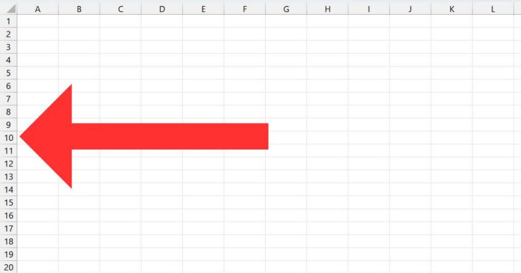
Select an entire column using the mouse

1. Move your mouse to the top of the column letter that you want to select.
   • (The column letters are located at the top of the worksheet.)
2. Click on the column letter.

The entire column will be selected, and it will be highlighted in blue.

Select an entire row using the keyboard

1. Move the active cell to any cell in the row you want to select.
2. Press the Shift key and the Spacebar at the same time.

The entire row will be selected, and it will be highlighted in blue.

Select an entire column using the keyboard

1. Move the active cell to any cell in the column that you want to select.
2. Press the Ctrl key and the Spacebar at the same time on Windows. Or the Command key and the Spacebar at the same time on Mac.

The entire column will be selected, and it will be highlighted in blue.

To deselect a row or column you have selected.

Click on any cell outside of the selected row or column, or press the Esc key on your keyboard.

The selected row or column will no longer be highlighted.

Selecting Non-contiguous Ranges

In Excel, you can select non-contiguous ranges of cells (i.e., cells that are not next to each other). Using either the mouse or the keyboard.

Here’s how to do it:

Select a non-contiguous range of cells using the mouse

1. Click on the first cell in the range that you want to select.
2. Hold down the Ctrl key on Windows or the Command key on Mac.
3. Click on each additional cell you want to include in the range.
4. Release the Ctrl or Command key when you have selected all the cells that you want to include in the range.

The selected cells will be highlighted in blue, but they will not be adjacent to each other.

Select a non-contiguous range of cells using the keyboard

1. Move the active cell to the first cell in the range that you want to select.
2. Press and hold down the Ctrl key on Windows or the Command key on Mac.
3. Use the arrow keys to move to the next cell or range of cells that you want to include in the selection.
4. Press the Spacebar to add the current cell or range to the selection.
5. Release the Ctrl or Command key when you have selected all the cells that you want to include in the range.

The selected cells will be highlighted in blue, but they will not be adjacent to each other.

To deselect a non-contiguous range of cells, press the Esc key on your keyboard or click on any cell outside the selected range.

The selected cells will no longer be highlighted.

Select a named ranges using the mouse

In Excel, you can select named ranges using either the mouse or the keyboard.

Here’s how to do it:

To select a named range using the mouse:

1. Click on any cell within the named range that you want to select.
2. Go to the Formulas tab on the ribbon and click on the Name Manager button.
3. In the Name Manager dialog box, locate the named range you want to select and click on it to highlight it.
4. Click on the “Edit…” button to open the Edit Name dialog box.
5. In the Edit Name dialog box, click on the “OK” button.

The named range will be selected, and it will be highlighted in blue.

Select a named range using the keyboard

1. Press the F5 key on your keyboard to open the Go To dialog box.
2. In the Go To dialog box, type in the name of the named range that you want to select.
3. Click on the “OK” button.

The named range will be selected, and it will be highlighted in blue.

Once you have selected a named range, you can perform various operations, such as copying, formatting, or applying formulas.

To deselect a named range, click on any cell outside the selected range, or press the Esc key on your keyboard.

The named range will no longer be highlighted.

Working with Ranges in Excel

Formatting a Range

Formatting a range in Excel allows you to change the appearance of the selected cells, including font style, font size, cell borders, background color, and more. Here’s how to format a range in Excel:

1. Select the range of cells that you want to format.
2. Go to the Home tab on the ribbon and click on the drop-down arrow next to any formatting button, such as the Font or Fill Color button.
3. Choose the formatting options that you want to apply to the selected cells.

For example, you can choose a different font style, font size, font color, or cell background color.

• To add cell borders, go to the Home tab on the ribbon and click on the Borders button. Choose the type of border that you want to add, such as a solid line or a dotted line, and select the cells where you want to add the border.

• To apply a cell style, go to the Home tab on the ribbon and click on the Cell Styles button. Choose a style from the list of available styles, and the selected cells will be formatted accordingly.

You can also use the Format Cells dialog box to format a range in Excel.

To do this:

1. Select the range of cells that you want to format.
2. Right-click on the selected cells and choose “Format Cells” from the context menu.
3. In the Format Cells dialog box, choose the formatting options that you want to apply to the selected cells, such as font style, font size, cell border, or number format.
4. Click on the “OK” button to apply the formatting to the selected cells.

Formatting a range in Excel can help you to make your data more visually appealing and easier to read. You can experiment with different formatting options to find the style that works best for your data.

Inserting Data into a Range

To insert data into a range in Excel, follow these steps:

1. Select the cell or cells where you want to insert the data.
2. If you want to insert data into multiple cells, select the range of cells.
3. Type the data into the selected cell(s).
4. Press Enter to move to the next cell down or to the right, depending on the direction of the selection.

If you want to insert data into multiple cells at once, you can select the cells and then type the data into the formula bar at the top of the worksheet.

To do this, select the cells, click in the formula bar, type the data, and then press Ctrl + Enter.

If you want to insert data into a specific location within a range, you can use the Insert Cells command.

Here’s how:

1. Select the cell or cells where you want to insert the data.
2. Right-click on the selected cell(s) and choose “Insert” from the context menu.
3. In the Insert dialog box, choose the type of insertion you want to make, such as shifting cells down or shifting cells to the right.
4. Click on the “OK” button to insert the cells and create space for the new data.
5. Type the data into the newly inserted cells.

You can also insert data into a range by copying and pasting.

To do this:

1. Select the cells that contain the data you want to copy.
2. Press Ctrl + C to copy the data.
3. Select the cell or cells where you want to insert the data.
4. Right-click on the selected cell(s) and choose “Paste” from the context menu.
5. Choose the type of paste you want to make, such as values, formulas, or formatting.
6. Click on the “OK” button to paste the data into the selected cells.

Inserting data into a range in Excel is a basic operation that is necessary for creating and editing spreadsheets.

With these simple steps, you can insert data quickly and easily, whether you’re entering data manually, inserting new cells, or copying and pasting.

Deleting Data from a Range

Deleting data from a range in Excel is a common task that can be done in several ways.

Here are some methods to delete data from a range:

• Delete a single cell: Select the cell that you want to delete, then press the Delete key on your keyboard. This will delete the contents of the cell, but not the cell itself.

• Delete a range of cells: Select the range of cells that you want to delete, then press the Delete key on your keyboard. This will delete the contents of all selected cells, but not the cells themselves.

• Clear cell contents: Select the cell or range of cells that you want to clear, then right-click and choose “Clear Contents” from the context menu. This will delete the contents of the selected cells, but not the formatting or any comments.

• Clear all: Select the cell or range of cells that you want to clear, then right-click and choose “Clear All” from the context menu. This will delete the contents, formatting, and comments from the selected cells.

• Use the Delete command: Select the cell or range of cells that you want to delete, then right-click and choose “Delete” from the context menu. In the Delete dialog box, choose the type of deletion you want to make, such as shifting cells up or shifting cells to the left. Click on the “OK” button to delete the cells and remove them from the worksheet.

Deleting data from a range in Excel is a quick and easy task, and can be done using a variety of methods depending on your needs.

Selecting the cells or range that you want to delete. You can quickly clear unwanted data or create space for new data in your spreadsheet.

Copying and Pasting a Range

Copying and pasting a range in Excel is a useful feature. That allows you to quickly duplicate data within a worksheet or between different worksheets.

Here’s how to copy and paste a range in Excel:

1. Select the range of cells that you want to copy.
   • You can do this by clicking and dragging over the cells, or by clicking on the first cell and then holding down the Shift key while clicking on the last cell in the range.
2. Right-click on the selected cells and choose “Copy” from the context menu, or press Ctrl + C on your keyboard.
   • This will copy the contents of the cells to the clipboard.
3. Move your cursor to the location where you want to paste the copied cells, and then right-click and choose “Paste” from the context menu, or press Ctrl + V on your keyboard.

This will paste the contents of the clipboard into the selected cells.

By default, Excel will paste the copied cells into the same location as they were copied from.

However, you can also paste the cells into a different location by selecting the destination cells before pasting.

You can also use the “Paste Special” command to paste only certain elements of the copied cells, such as values, formulas, or formatting.

To access this command, right-click on the destination cells and choose “Paste Special” from the context menu.

In the “Paste Special” dialog box, choose the type of paste you want to make and then click on the “OK” button.

Copying and pasting a range in Excel is a quick and easy way to duplicate data and save time when working with large spreadsheets. By mastering this technique, you can become more efficient and productive in your Excel workflow.

Moving a Range

Moving a range in Excel means that you are relocating a selected group of cells from one area of a worksheet to another area.

This can be useful when you want to rearrange the layout of your data, or when you need to make room for new data in a particular area.

Here’s how to move a range in Excel:

1. Select the range of cells that you want to move.
   • You can do this by clicking and dragging over the cells, or by clicking on the first cell.
2. Then holding down the Shift key while clicking on the last cell in the range.
3. Move your cursor to the border of the selected cells until you see a four-headed arrow icon.
4. Click and hold the left mouse button to drag the cells to their new location.
5. Release the left mouse button once you have positioned the cells in their new location.
6. If you want to overwrite the existing data in the destination cells, release the left mouse button while holding down the Shift key.
   • If you want to insert the cells into the new location without overwriting any existing data, release the left mouse button while holding down the Ctrl key.
7. Finally, release the Shift or Ctrl key, and the cells will be moved to their new location.

Moving a range in Excel is a simple process. But it’s important to be careful when moving data to avoid accidentally overwriting or deleting important information.

It’s a good idea to make a backup of your spreadsheet before moving any large ranges. To double-check that the cells are in the correct location before finalizing the move.

Sorting a Range

Sorting a range in Excel means arranging the data in a specific order based on the values in one or more columns.

This is a useful feature when you need to quickly analyze and organize large sets of data. Here’s how to sort a range in Excel:

1. Select the range of cells that you want to sort.
   • You can do this by clicking and dragging over the cells, or by clicking on the first cell and then holding down the Shift key while clicking on the last cell in the range.
2. Go to the “Data” tab in the Excel ribbon and click on the “Sort” button.
   • This will open the “Sort” dialog box.
3. In the “Sort” dialog box, choose the column that you want to sort by from the “Sort by” drop-down list.
   • You can also choose a secondary column to sort by, if necessary.
4. Choose the sort order from the “Order” drop-down list.
   • You can sort in ascending (smallest to largest) or descending (largest to smallest) order.
5. If your data includes headers, make sure to check the “My data has headers” box to avoid sorting the headers along with the data.
6. Click on the “OK” button to apply the sort.

Excel will then rearrange the data in the selected range based on the chosen sorting criteria.

If you want to undo the sort or change the sort criteria, you can use the “Undo” button or reopen the “Sort” dialog box and make adjustments.

Sorting a range in Excel is a powerful tool that can help you quickly analyze and organize large sets of data. By mastering this technique, you can become more efficient and productive in your Excel workflow.

Filtering a Range

Filtering a range in Excel means showing only specific rows of data that meet certain criteria while hiding the other rows. This is a useful feature when you need to focus on specific data or perform analysis on a subset of data.

Here’s how to filter a range in Excel:

1. Select the range of cells that you want to filter.
   • You can do this by clicking and dragging over the cells, or by clicking on the first cell and then holding down the Shift key while clicking on the last cell in the range.
2. Go to the “Data” tab in the Excel ribbon and click on the “Filter” button.
   • This will add drop-down arrows to the headers of your data.
3. Click on the drop-down arrow in the header of the column that you want to filter.
   • This will open the filter menu.
4. In the filter menu, you can choose to filter by specific values, ranges of values, or conditions such as “greater than” or “less than”.
   • You can also use search and sorting options to help you find the data you need.
5. After choosing your filter criteria, click on the “OK” button to apply the filter.
   • Excel will then hide any rows of data that do not meet the selected criteria, leaving only the filtered data visible.
6. If you want to remove the filter and show all the data again, simply go to the “Data” tab in the Excel ribbon and click on the “Clear” button.

Filtering a range in Excel is a powerful tool that can help you focus on specific data. Making more informed decisions based on that data.

By mastering this technique, you can become more efficient and productive in your Excel workflow.

Using Formulas with a Range

Using formulas with a range in Excel means performing calculations on a set of data within a range of cells.

This is a useful feature when you need to perform complex calculations or manipulate data in a specific way.

Here’s how to use formulas with a range in Excel:

• Select the range of cells that you want to use in your formula. You can do this by clicking and dragging over the cells, or by clicking on the first cell and then holding down the Shift key while clicking on the last cell in the range.
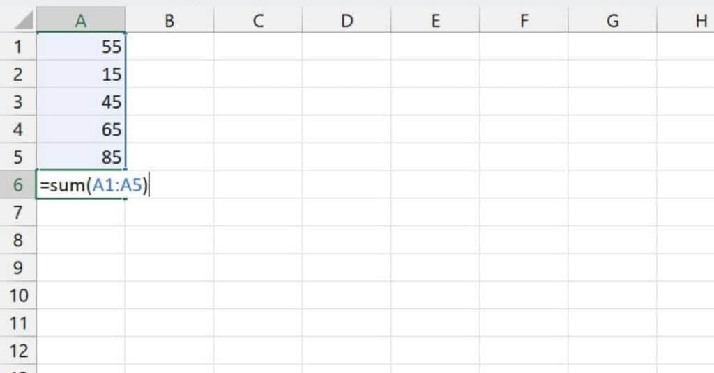
• Type your formula into the formula bar at the top of the Excel window. Make sure to include the appropriate range references in your formula. For example, if you want to add up the values in cells A1 through A5, your formula might look like this: =SUM(A1:A5)
• Press Enter to apply the formula to the selected range of cells. Excel will automatically calculate the result of the formula and display it in the cell where you typed the formula.

You can use a wide range of formulas with a range in Excel, including basic arithmetic formulas such as addition, subtraction, multiplication, and division, as well as more complex formulas that involve functions, logical operators, and more.

By mastering the use of formulas with a range, you can become more efficient and productive in your Excel workflow and perform complex calculations with ease.

Advanced Techniques for Working with Ranges in Excel

Using Range Names in Formulas

Using range names in formulas in Excel can make your formulas easier to read, understand, and manage.

Range names are user-defined names that represent a range of cells in a worksheet.

Instead of referring to a range of cells by its cell references (e.g. A1:B10), you can give it a name (e.g. Sales_Data) and refer to it by that name in your formulas.

Here’s how to use range names in formulas in Excel:

• Select the range of cells that you want to name. You can do this by clicking and dragging over the cells, or by clicking on the first cell and then holding down the Shift key while clicking on the last cell in the range.
• Go to the “Formulas” tab in the Excel ribbon and click on the “Define Name” button. This will open the “New Name” dialog box.
• In the “New Name” dialog box, type the name that you want to give to the range in the “Name” field. Make sure the “Refers to” field displays the correct cell range, or enter the correct cell range if it doesn’t.
• Click on the “OK” button to save the range name.
• Now you can use the range name in your formulas.

For example, if you named a range “Sales_Data” and you want to calculate the average of the values in that range, you can use the following formula: =AVERAGE(Sales_Data)

Using range names in formulas can make your formulas more concise and easier to read.

Named ranges can also be useful when working with large or complex worksheets. As they can make it easier to refer to specific ranges of cells without needing to remember the cell references.

In addition, named ranges can be easily updated if the range of cells they refer to changes, simply by editing the “Refers to” field in the “Define Name” dialog box.

Instead of updating the cell references in all your formulas, you only need to update the range name once.

By mastering the use of range names in formulas, you can become more efficient and productive in your Excel workflow.

Working with Dynamic Ranges

Working with dynamic ranges in Excel means using formulas and functions that adjust to include new data that is added to or removed from a range.

Dynamic ranges are useful when you have data that is frequently updated or when you want to make sure that your formulas always include the most up-to-date data.

Here are some ways to work with dynamic ranges in Excel:

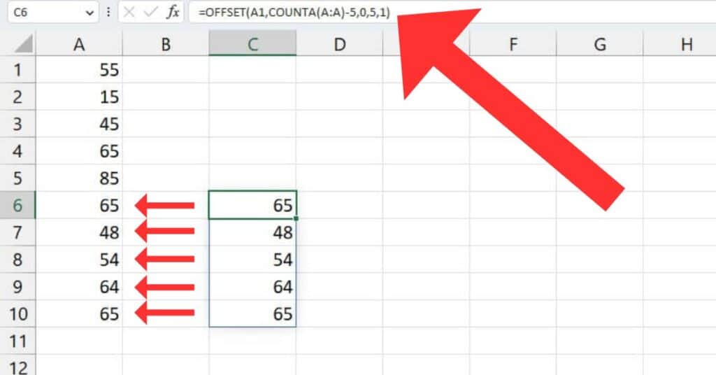
• Using the OFFSET function: The OFFSET function is a powerful function that allows you to define a range that adjusts dynamically based on the number of rows and columns you specify.

For example, if you want to create a range that always includes the last 5 rows of data in a worksheet, you can use the OFFSET function in combination with the COUNTA function, like this:

=OFFSET(A1,COUNTA(A:A)-5,0,5,1).

This formula starts at cell A1 and then counts the number of non-blank cells in column A, subtracts 5 from that number, and creates a range that includes the last 5 rows of data.

Creating Tables from Ranges

Creating tables from ranges in Excel is a useful way to organize and analyze data. Tables provide several advantages, such as automatic formatting, filtering, sorting, and summarizing data.

Here’s how to create tables from ranges in Excel:

1. Select the range: First, select the range of cells you want to turn into a table. The range can include headers, data, and totals.
2. Create a table: With the range selected, go to the “Insert” tab on the ribbon and click on the “Table” button.
3. Excel will automatically detect the range and display the “Create Table” dialog box.
4. Check the table range: In the “Create Table” dialog box, make sure the range of cells is correct.
5. Excel will usually detect the range automatically, but you can adjust it manually if necessary.
6. Choose a table style: Select a table style from the gallery of options in the “Create Table” dialog box. You can also customize the table style by selecting “New Table Style” at the bottom of the gallery.
7. Check the “My table has headers” box: If your range includes headers, make sure to check the “My table has headers” box in the “Create Table” dialog box. This will tell Excel to use the first row of the range as the column headers for the table.
8. Click “OK”: Once you have selected a table style and checked the options, click the “OK” button to create the table.

Excel will format the range as a table, and you can start working with the table features.

After you create a table, Excel will automatically add filter controls to each column header, which allows you to filter the data in the table based on specific criteria.

You can also sort the data in the table by clicking on the column headers, and Excel will display a summary of the data in the “Total” row at the bottom of the table.

Additionally, you can use formulas and functions with tables, which will automatically adjust as you add or remove data from the table.

Creating tables from ranges in Excel can make it easier to analyze and manage data, especially when working with large datasets.

The next logical step from here is to go into a little more detail in a more focused subject. I have the perfect section for you and that is my Excel Basics page. If you are a beginner or a excel expert there will be something for you to learn in this section.

If you prefer to watch excel demonstrations then I have put together a YouTube channel that is well worth checking out if video is your thing.