How to Hide Columns in Excel

In this short tutorial, I’m going to show you how to hide columns in an Excel spreadsheet.

It’s simple and easy!

By doing this, you’ll be able to hide any information that you don’t want to share in the table.

Let’s get started!

Watch this video on YouTube.

Highlighting Columns in Excel

There are a couple of different ways to hide columns in a spreadsheet.

I’ll show you two of them.

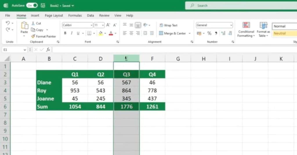
First, highlight the column that you’d like to hide by clicking on the bar of letters and selecting the relevant column.

If there are multiple columns that you want to hide, press the Shift key and click on each of the columns.

If the columns you want to hide are not consecutive, press the Ctrl key instead of Shift.

First Way How to Hide Columns in Excel

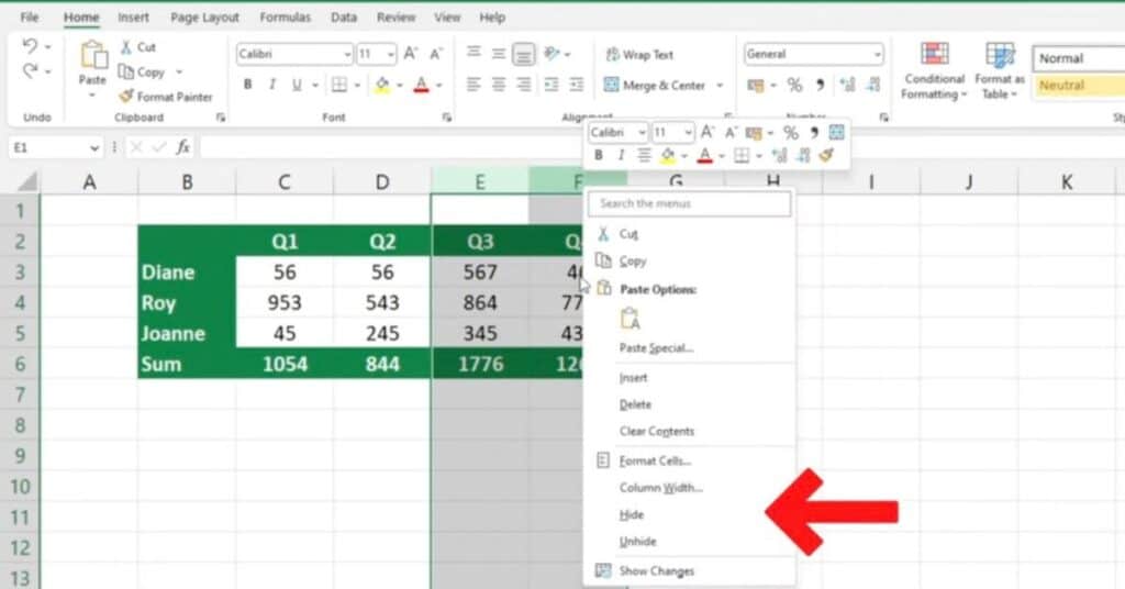
Once you’ve selected all of the necessary columns, right-click and select the “Hide” option.

The hidden columns will no longer be visible in the table on the screen or if you try to print out the spreadsheet.

Don’t worry though, they’re not gone for good!

You can always unhide them later.

Second Way How to Columns Rows in Excel

Now let’s try the other way to hide columns.

Select the columns again, this time by dragging.

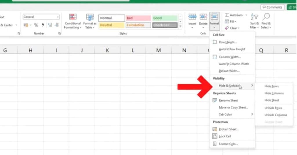
Then go to the Home tab, select the Cells section (or group), and click the Format button to get the Format menu.

Find the Hide and Unhide options and select Hide Columns.

And you’re done!

You have learned How to Hide Columns in Excel.

To learn how to unhide columns in Excel, see the next tutorial from Sheet Leveller.

If you found this tutorial helpful, and if you want to learn Excel our complete guide section is the place to go that will help you use Excel like a boss!

If you want to master the excel functions then head over to our excel function section that will help you with them. We even have a dedicated section for Excel Formulas.

Thanks for reading, see you at the next one!

How to Hide Columns in Excel | Beginner’s Guide