Excel LOOKUP Function is one of the most useful functions in Excel that helps to search for a value in a dataset and return a corresponding value from the same or a different location. This function is widely used for data analysis and management tasks in various industries such as finance, marketing, and human resources. The LOOKUP function is often used in combination with other Excel functions such as VLOOKUP and HLOOKUP to perform more complex tasks.
Excel LOOKUP Function Summary
Excel LOOKUP function searches for a value in a vector or array and returns a corresponding value from the same position in another vector or array. It can be used with different lookup methods like exact match, approximate match, or wildcard.
LOOKUP Function Purpose
The purpose of the Excel LOOKUP function is to search for a specific value in a given range or array and return a corresponding value from the same or a different location.
LOOKUP Function Arguments
The LOOKUP function takes two or three arguments:
- Lookup_value: The value to be searched for in the dataset.
- Lookup_vector: The range of cells or array where the value should be searched for.
- [Result_vector]: An optional argument that specifies the range of cells or array from which the corresponding value should be returned.
LOOKUP Function Return Value
The Excel LOOKUP function returns the corresponding value from the same or a different location in the dataset.
LOOKUP Function Syntax
The syntax for the Excel LOOKUP function is as follows:
=LOOKUP(lookup_value,lookup_vector,[result_vector])Excel LOOKUP Function Examples
Excel’s LOOKUP function is a powerful tool that helps you find specific data within a large data set. Here are some examples of how you can use the LOOKUP function in your spreadsheets.
Using LOOKUP with an exact match
Suppose you have a table of student grades, and you want to look up the grade for a specific student. You could use the LOOKUP function like this:
=LOOKUP("John",A2:A10,B2:B10)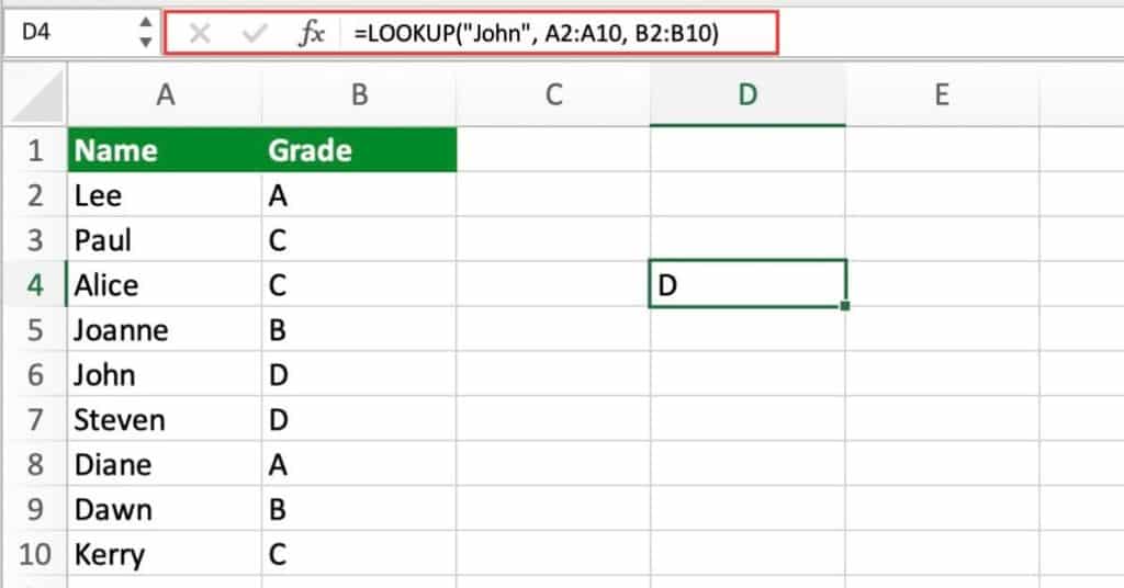
In this example, “John” is the value you’re looking up, and A2:A10 is the range of cells that contains the student names. B2:B10 is the range of cells that contains the corresponding grades. The LOOKUP function will find the row where “John” appears in column A, and return the corresponding value in column B (which is Alice’s grade).
Using LOOKUP with an approximate match
Suppose you have a list of employee salaries, and you want to look up the salary for an employee based on their years of experience. You could use the LOOKUP function like this:
=LOOKUP(5,B2:B10,C2:C10)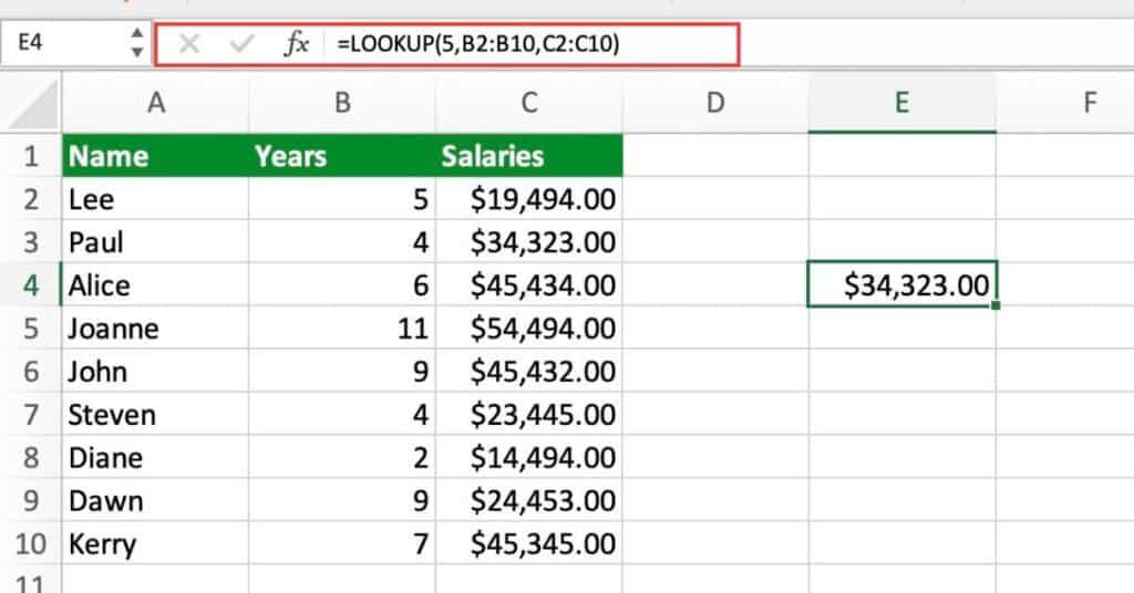
In this example, 5 is the value you’re looking up (which represents the number of years of experience). B2:B10 is the range of cells that contains the years of experience, and C2:C10 is the range of cells that contains the corresponding salaries. The LOOKUP function will find the largest value in column B that is less than or equal to 5 (which would be 4 in this case), and return the corresponding salary from column E.
Using LOOKUP with a vector array
Suppose you have a vector array of numbers, and you want to find the value that is closest to a specific target value. You could use the LOOKUP function like this:
=LOOKUP(0.5,{0.1,0.2,0.3,0.4,0.5,0.6,0.7,0.8,0.9,1.0})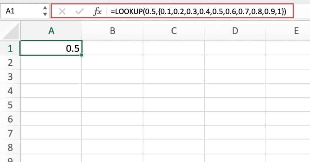
In this example, 0.5 is the target value you’re looking for, and the array {0.1,0.2,0.3,0.4,0.5,0.6,0.7,0.8,0.9,1.0} is the range of values to search through. The LOOKUP function will find the value in the array that is closest to 0.5 (which would be 0.5 itself), and return that value.
Returning the Last Value in a Range
The LOOKUP function can also be used to return the last value in a range of data. In this example, we are looking up the last non-zero value in a column of data.
The formula would be:
=LOOKUP(2,1/(B2:B8<>0),B2:B8) 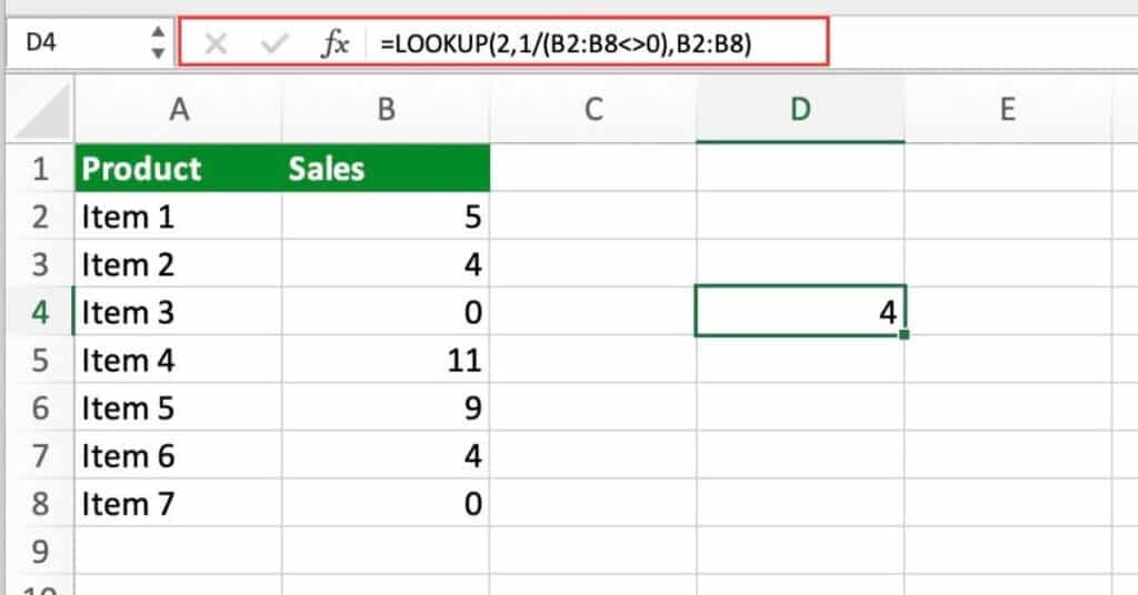
As we wanted to find the last non-zero value in the Sales column. In our example above we get a return of 4 as this is the last non-zero value in a column.
Performing a Two-Way Lookup
In Excel, a two-way lookup refers to a situation where you need to look up a value based on two criteria, such as finding the price of a particular product for a specific month. The LOOKUP function can be used to perform a two-way lookup in Excel.
Let’s say you have a table of sales data that contains sales amounts for different products and months.
The formula would be:
=INDEX(B2:B6,LOOKUP(D2,A2:A6))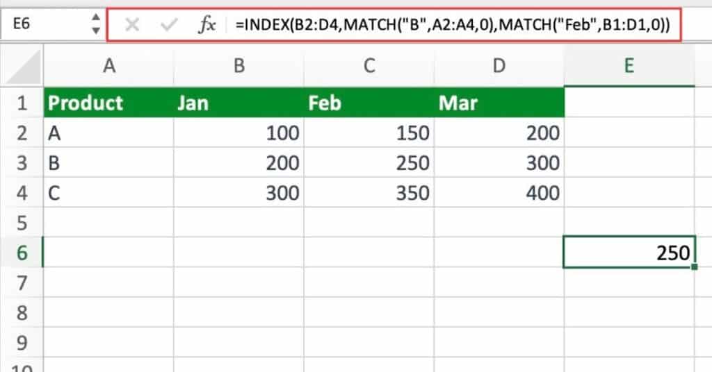
This formula uses the MATCH function to find the row and column numbers and then the INDEX function to return the value at the intersection of the row and column. The result of the formula would be 250, which is the sales amount for product B in February.
Looking Up Values in Multiple Columns
The LOOKUP function in Excel can be used to look up values in multiple columns of a table. This is useful when you have a large table and you want to find a specific value based on more than one criterion.
Suppose you have a table with three columns: Product, Color, and Price. You want to find the price of a product with a specific color.
You can use the following formula:
=LOOKUP(D2&E2,A2:A8&B2:B8,C2:C8)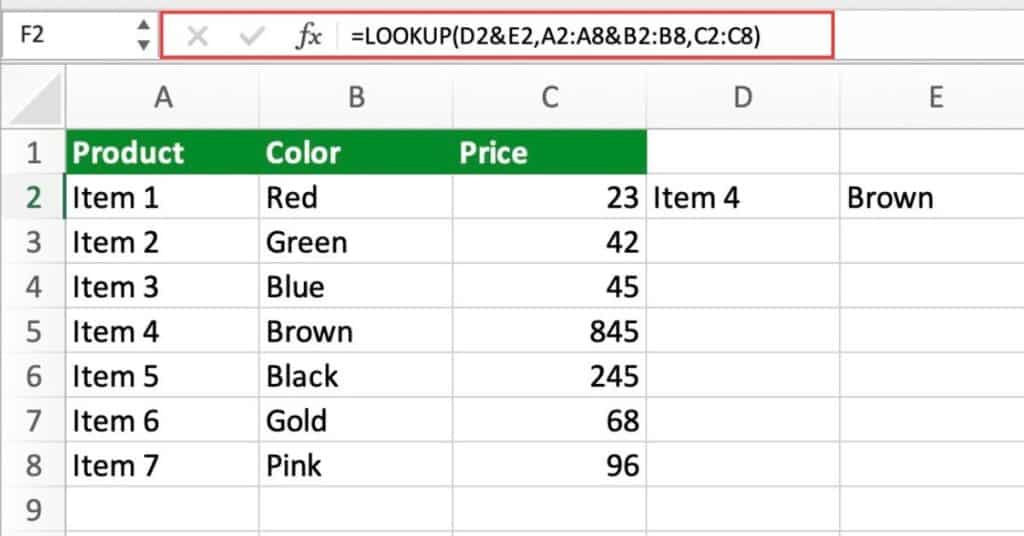
The corresponding value in column C is returned as the result.
These are just a few examples of how you can use the Excel LOOKUP function. Keep in mind that the LOOKUP function has some limitations. With them it may not always be the best option for your data analysis needs. Also note that starting with Excel 2019. The LOOKUP function has been replaced by the more powerful and flexible XLOOKUP function.
Excel LOOKUP Function Notes
- The LOOKUP function requires that the lookup_vector be sorted in ascending order.
- If the lookup_value is not found in the lookup_vector, the function returns an error value.
- If the lookup_value is found more than once in the lookup_vector, the function returns the last matching value.
