Excel TRANSPOSE Function is a powerful tool used to transform data from rows to columns and columns to rows. It helps in rearranging the data in a more meaningful way, especially when dealing with large data sets. By using this function, users can quickly switch the orientation of their data, making it more readable and easier to analyze.
TRANSPOSE Function Summary
The TRANSPOSE function is a powerful Excel tool that can quickly convert vertical ranges to horizontal ones, or vice versa. To use the TRANSPOSE function effectively, it’s important to enter it as an array formula in a range with the same number of rows and columns as the source range. This way, you can transform your data with ease and streamline your work.
TRANSPOSE Function Purpose
The main purpose of the Excel TRANSPOSE function is to transpose a range of cells from columns to rows or vice versa.
TRANSPOSE Function Arguments
The only argument for the Excel TRANSPOSE function is the range of cells that the user wants to transpose. This range can be a single row, single column, or a rectangular block of cells.
TRANSPOSE Function Return Value
The Excel TRANSPOSE function returns a transposed range of cells, meaning that the columns of the original range become rows, and the rows become columns.
TRANSPOSE Function Syntax
=TRANSPOSE(array)TRANSPOSE Function Examples
In this section, we’ll explore some practical examples of the TRANSPOSE function in action. You’ll learn how to use this powerful Excel function to quickly and easily reorganize your data from rows to columns or vice versa. Whether you’re working with small data sets or large data tables, the TRANSPOSE function can save you time and help you gain valuable insights from your data.
TRANSPOSE Vertical Range
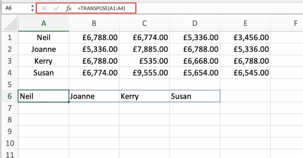
When a vertical range is given as input, the function returns a horizontal range.
Suppose we have a table with the data of students’ marks in different subjects. We want to transpose this data from columns to rows.
To do this, we can use the TRANSPOSE function as follows:
=TRANSPOSE(A1:A4)
This will transpose the range A1:A4 and return the result in a new range of cells.
TRANSPOSE Horizontal Range
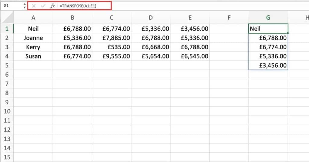
When a horizontal range is given as input, the function returns a vertical range.
Suppose we have a table with the data of students’ marks in different subjects, but this time the data is in rows. We want to transpose this data from rows to columns. To do this, we can use the TRANSPOSE function as follows:
=TRANSPOSE(A1:E1)
This will transpose the range A1:E1 and return the result in a new range of cells.
TRANSPOSE With XLOOKUP
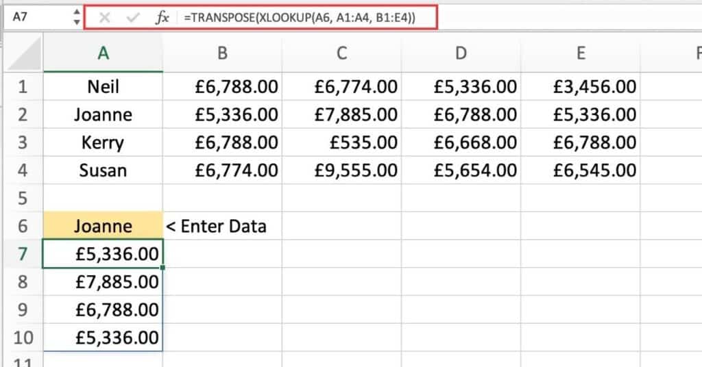
I’ll show you how to use the TRANSPOSE and XLOOKUP functions together to perform a lookup and transpose the result.
Here’s an example of the function we’ll be using:
=TRANSPOSE(XLOOKUP(A6, A1:A4, B1:E4))
Let’s break down the function and see what’s happening:
- A6 is the value we’re looking for in the range A1:A4.
- A1:A4 is the range we’re searching for the value in.
- B1:E4 is the range where we want to return the corresponding values.
- XLOOKUP(A6, A1:A4, B1:E4) searches for the value in A6 in the range A1:A4 and returns the corresponding values in the range B1:E4.
- TRANSPOSE(XLOOKUP(A6, A1:A4, B1:E4)) then flips the result from vertical to horizontal, or vice versa, depending on the orientation of the original ranges.
The result of the function will be a horizontal array of values that correspond to the lookup value A6.
Using Paste Special with Transpose to Convert Data in Excel
While the TRANSPOSE function is great for creating dynamic solutions that update automatically when source data changes, it may not be the most efficient option if you only need a one-time conversion. In such cases, you can use the Paste Special feature and select the Transpose option to achieve the desired result.
To use Paste Special with Transpose:
- Copy the data range that you want to transpose.
- Select the cell where you want to paste the transposed data.
- Right-click the cell and select “Paste Special” from the context menu.
- In the Paste Special dialog box, select the “Transpose” option.
- Click “OK” to paste the transposed data.
Note that when using this method, you’re not creating a dynamic range like you would with the TRANSPOSE function. The transposed data will remain static, and won’t update if the source data changes.
In some cases, using Paste Special with Transpose can be quicker and easier than using the TRANSPOSE function. Additionally, if you’re working with a large dataset, using the Paste Special feature may be faster than waiting for Excel to calculate the TRANSPOSE function.
Overall, using Paste Special with Transpose is a simple and effective way to convert data in Excel, especially when you don’t need a dynamic solution.
TRANSPOSE Function Notes
- The Excel TRANSPOSE function only works with a range of cells, not individual cells.
- The size of the transposed range must match the size of the original range.
- If the original range contains any blank cells, they will be included in the transposed range as well.
- The transposed range is a static view of the original data, and any changes made to the original data will not be reflected in the transposed range unless the function is re-applied.
